以在 GitHub 上执行或查看/下载此笔记本

分析用于病理的声学特征

此笔记本对一些语音样本进行了简单的语音分析。如果你是语音特征提取的新手，我们建议在阅读本笔记本之前先阅读 Aalto 语音处理第三章基本表示，以理解此处使用的信号处理技术背后的背景和理论。在整个教程中，多次提到了 PRAAT 软件，它是一个早期的开源软件，用于计算这些度量，我们有时会将我们的结果与它进行比较。你可以在此处找到更多信息

• https://www.fon.hum.uva.nl/praat/

为了演示目的，我们首先下载一个来自帕金森病患者的公开样本，并将其裁剪至仅包含持续发声的部分。

%%capture
!wget -O BL01_ENSS.wav "https://data.mendeley.com/public-files/datasets/9dz247gnyb/files/5183cb8f-77ff-418d-a4cc-e2eca48cb6a5/file_downloaded"
!ffmpeg -ss 18 -t 3.5 -y -i BL01_ENSS.wav phonation.wav

%%capture
import torch
import torchaudio
import matplotlib.pyplot as plt
from speechbrain.processing.vocal_features import *

# Load sustained phonation recording from QPN dataset
audio_filename = "phonation.wav"
audio, sample_rate = torchaudio.load(audio_filename)

# Parameters for all figures in the document
plt.rcParams["figure.figsize"] = (14,2)
plt.rcParams['axes.xmargin'] = 0

# Downsample to reduce number of points on the plot
downsample_factor = 20
xs = torch.arange(len(audio[0,::downsample_factor])) / sample_rate * downsample_factor
plt.plot(xs, audio[0,::downsample_factor], linewidth=.5)
plt.xlabel("Time [s]")
plt.ylabel("Amplitude")
plt.show()

介绍

为了理解这种语音分析的工作原理，我们将逐步介绍声学特征计算函数，包括

• speechbrain.processing.vocal_features.compute_autocorrelation_features

• speechbrain.processing.vocal_features.compute_periodic_features

• speechbrain.processing.vocal_features.compute_gne

这些不同的声学特征处理方法可以为潜在的声带病变提供不同的指示，我们将在教程中进行解释。我们首先设置适用于所有部分的基本参数。

# Frequency of human speech is usually between 75-300 Hz
min_f0_Hz = 80
max_f0_Hz = 300

# A new window of 0.05 second length every 0.01 seconds
step_size = 0.01
window_size = 0.05

# Do some number manipulations
step_samples = int(step_size * sample_rate)
window_samples = int(window_size * sample_rate)
max_lag = int(sample_rate / min_f0_Hz)
min_lag = int(sample_rate / max_f0_Hz)

print("Samples between (the start of) one frame and the next:", step_samples)
print("Samples contained within each frame:", window_samples)
print("Number of samples in the maximum lag:", max_lag)
print("Number of samples in the minimum lag:", min_lag)

Samples between (the start of) one frame and the next: 441
Samples contained within each frame: 2205
Number of samples in the maximum lag: 551
Number of samples in the minimum lag: 147

我们对这些值的合理性检查是，帧中至少包含一个完整周期（对于最低 Hz），最多包含 8 个（对于最高 Hz）。

计算自相关和相关特征

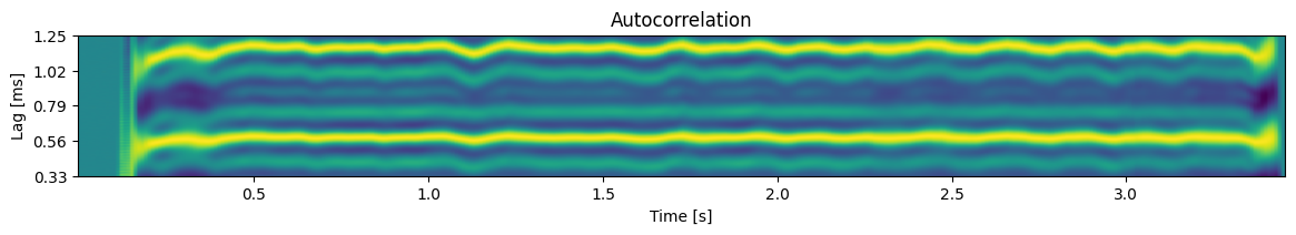
第一组特征，自相关特征，可以捕捉因气声/嘈杂/不规则发声而产生的病变迹象。原因通常是对发声的某些方面（例如声带）控制不足，导致周期变得不那么规则。

自相关是信号在从 min_lag 到 max_lag 的每个滞后处与自身的互相关。最小滞后和最大滞后对应于人类发声范围的极端——以减少在不可能对应于人类发声频率的频率处出现假峰的可能性。对于所有周期性/谐波信号（包括发声），在对应于信号周期的规则滞后间隔处存在峰值。谐波性是最大峰值与滞后为零时出现的理论最大值（因为信号在滞后 0 时与自身完美对齐）之比。

谐波性是衡量病变的一个有用指标，因为任何不规则性都会表现为信号与时间偏移版本互相关得分的降低。

对于可能有助于理解自相关概念的动画，请参阅以下链接

• https://tahull.github.io/blog/2020/08/acf-animated

• https://github.com/chautruonglong/Fundamental-Frequency

# Split into frames, and compute autocorrelation for each frame
frames = audio.unfold(-1, window_samples, step_samples)
autocorrelation = autocorrelate(frames)

# Use autocorrelation maxima to compute harmonicity (max) and lags (index) corresponding to estimated period
harmonicity, lags = autocorrelation[:, :, min_lag:max_lag].max(dim=-1)
lags = torch.nn.functional.pad(lags, pad=(3, 3))

# Take the median of 7 frames to avoid short octave jumps
best_lags, _ = lags.unfold(-1, 7, 1).median(dim=-1)

# Re-add the min_lag back in after previous step removed it
best_lags = best_lags + min_lag
estimated_f0 = sample_rate / best_lags

xs = torch.arange(len(harmonicity[0])) * step_size

# Show autocorrelation from min lag to max lag
plt.imshow(autocorrelation[0, :, min_lag:max_lag].transpose(0,1), aspect=0.1, origin="lower")
plt.title("Autocorrelation")
plt.ylabel("Lag [ms]")
plt.xlabel("Time [s]")
xticks = (torch.arange(1, 7) / 2 / step_size).int().tolist()
plt.xticks(xticks, xs[xticks].tolist())
yticks = torch.linspace(0, max_lag - min_lag, 5).int()
plt.yticks(yticks.tolist(), ((yticks + min_lag) / step_samples).numpy().round(decimals=2))
plt.show()

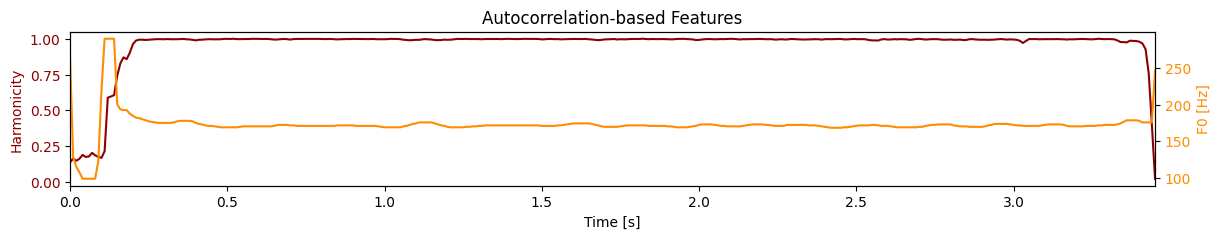
# Show autocorrelation-based features, harmonicity (usually represented in log scale as HNR) and f0
fig, ax1 = plt.subplots()
ax1.set_title("Autocorrelation-based Features")
ax1.set_ylabel("Harmonicity", color="darkred")
ax1.set_xlabel("Time [s]")
ax1.plot(xs, harmonicity[0], color="darkred")
ax1.tick_params(axis="y", labelcolor="darkred")
ax2 = ax1.twinx()
ax2.set_ylabel("F0 [Hz]", color="darkorange")
ax2.plot(xs, estimated_f0[0], color="darkorange")
ax2.tick_params(axis="y", labelcolor="darkorange")
plt.show()

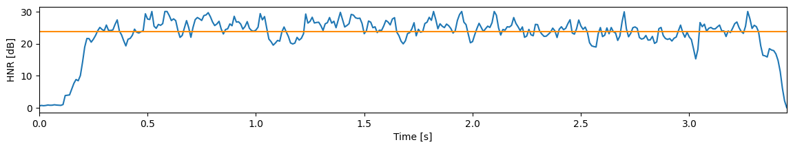
为了测量谐波噪声比 (HNR)，除了我们早期对谐波性的估计之外，还需要估计噪声。根据以下出版物，我们可以将噪声估计为 1 - 谐波性，因为谐波性的任何降低都是由噪声引起的。

参见 J. Fernandez、F. Teixeira、V. Guedes、A. Junior 和 J. P. Teixeira 的文章“谐波噪声比测量 - 窗口和长度的选择”

然而，我们发现 HNR 主要受噪声项影响，因此为了效率和简单起见，我们仅将 -10 * log(噪声) 作为 HNR 值（以分贝为单位）。

HNR 的最大值为 30 dB，通过将噪声钳位到最小值 10^-3 来实现。

noise = torch.clamp(1 - harmonicity, min=10**-3)
hnr = -10 * torch.log10(noise)

plt.plot(xs, hnr[0])
plt.xlabel("Time [s]")
plt.ylabel("HNR [dB]")

# PRAAT uses harmonicity to determine voicing in this scenario
avg_hnr = hnr[harmonicity > 0.45].mean().numpy().round(decimals=1)
plt.axhline(y=avg_hnr, color="darkorange")
print("Average HNR:", avg_hnr)

Average HNR: 23.8

计算基于周期的特征

病变有时也会表现为声音周期的不规则性。在语音诊断文献中非常常用的两个特征是 jitter 和 shimmer。

你可以在这里找到一个很好的解释

https://speechprocessingbook.aalto.fi/Representations/Jitter_and_shimmer.html

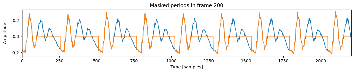
最基本的解释是，jitter 是周期长度波动的度量，而 shimmer 是周期峰值振幅波动的度量。

为了理解其工作原理，可视化单帧会有所帮助。我们使用第 200 帧，位于录音的 2.00 秒处。

我们将首先识别周期峰值，并屏蔽掉不在周期峰值 20% 范围内的所有内容，以避免从周期开始跳到周期中间。

frame_i = 200
plt.plot(frames[0, frame_i])

# Prepare for masking
masked_frames = torch.clone(frames).detach()
mask_indices = torch.arange(frames.size(-1)).view(1, 1, -1)
mask_indices = mask_indices.expand(frames.shape)
periods = best_lags.unsqueeze(-1)
period_indices = mask_indices.remainder(periods)

# Mask everything not within about 20% (1/5) of a period peak
jitter_range = periods // 5
peak, lag = torch.max(masked_frames, dim=-1, keepdim=True)
mask = (
    (period_indices < lag.remainder(periods) - jitter_range)
    | (period_indices > lag.remainder(periods) + jitter_range)
)
masked_frames[mask] = 0


plt.plot(masked_frames[0, frame_i])
plt.xlabel("Time [samples]")
plt.ylabel("Amplitude")
plt.title(f"Masked periods in frame {frame_i}")
plt.show()

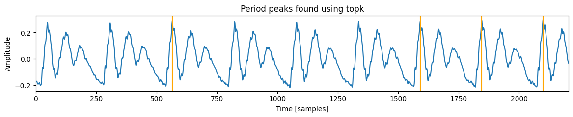
接下来，我们将识别用于计算 jitter 和 shimmer 的四个周期峰值。无论基频如何，我们都保持周期峰值数量一致，因为基频会影响窗口中出现的峰值数量。PRAAT 使用 3、5 或 7 个相邻峰值来计算 jitter 和 shimmer 的变体。该数量可以配置，但重要的是即使在最低频率下，也要保证窗口中有 4 个周期。

plt.plot(frames[0, frame_i])
peaks, lags = [], []

# Find neighboring peaks
peaks, lags = [], []
for i in range(4):
    peak, lag = torch.max(masked_frames, dim=-1, keepdim=True)
    mask = (
        (mask_indices > lag - periods // 2)
        & (mask_indices < lag + periods // 2)
    )
    masked_frames[mask] = 0
    peaks.append(peak.squeeze(-1))
    lags.append(lag.squeeze(-1))

peaks = torch.stack(peaks, dim=-1)
lags = torch.stack(lags, dim=-1)

for lag in lags[0, frame_i]:
    plt.axvline(lag, color="orange")

plt.title("Period peaks found using topk")
plt.xlabel("Time [samples]")
plt.ylabel("Amplitude")

print("Peak indices:", lags[0, 230])

Peak indices: tensor([ 437,  181, 1204,  693])

Jitter 是周期长度的平均变化。我们将每个周期的长度与整个窗口的周期估计值进行比较。平均差值即为 jitter，通过对周期进行归一化，得到一个介于 0 和 1 之间的数字。

lags = lags.remainder(periods)
jitter_frames = (lags - lags.float().mean(dim=-1, keepdims=True)).abs()
jitter = jitter_frames.mean(dim=-1) / best_lags

print("Peak lags from 0:", lags[0, frame_i])
print("Normalized period length differences:", jitter_frames[0, frame_i] / best_lags[0, frame_i])
print("Average jitter score for this frame:", jitter[0, frame_i])

Peak lags from 0: tensor([51, 53, 53, 55])
Normalized period length differences: tensor([0.0078, 0.0000, 0.0000, 0.0078])
Average jitter score for this frame: tensor(0.0039)

# PRAAT uses cutoff of jitter > 0.02 as un-voiced
plt.plot(xs, jitter[0] * 100)
plt.xlabel("Time [s]")
plt.ylabel("Jitter [%]")
plt.title("Jitter and average jitter score across full sample")
plt.axhline(y = jitter[jitter < 0.02].mean() * 100, color="darkorange")
plt.axvline(x = frame_i / 100, color="lightgrey")
print("Average Jitter: {0:.2f}%".format(100 * jitter[jitter < 0.02].mean().numpy()))

Average Jitter: 0.44%

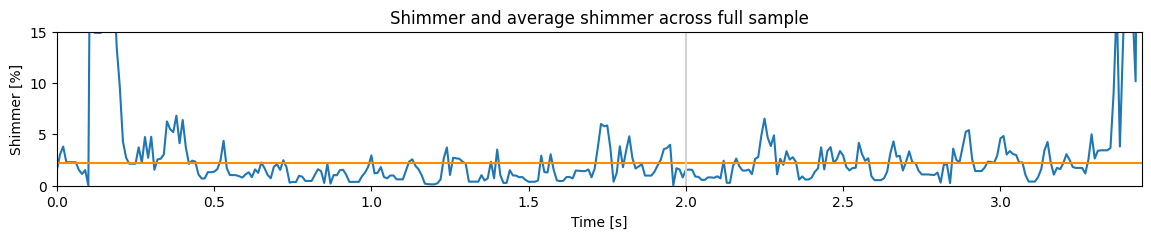
Shimmer 是峰值振幅的平均变化。我们首先计算每个峰值的振幅，然后计算每个峰值与平均峰值振幅的差值。Shimmer 就是平均差值通过总体平均振幅归一化后，得到一个介于 0 和 1 之间的分数。

avg_amps = peaks.mean(dim=-1, keepdims=True)
amp_diff = (peaks - avg_amps).abs()
shimmer = amp_diff.mean(dim=-1) / avg_amps.squeeze(-1).clamp(min=1e-3)

print("Normalized peak amplitude differences:", amp_diff[0, frame_i] / avg_amps[0, frame_i])
print("Shimmer score for the frame:", shimmer[0, frame_i])

Normalized peak amplitude differences: tensor([0.0294, 0.0015, 0.0098, 0.0210])
Shimmer score for the frame: tensor(0.0154)

# PRAAT uses jitter to determine if its voiced
plt.plot(xs, shimmer[0] * 100)
plt.xlabel("Time [s]")
plt.ylabel("Shimmer [%]")
plt.title("Shimmer and average shimmer across full sample")
plt.ylim((0, 15))
plt.axhline(y = shimmer[jitter < 0.02].mean() * 100, color="darkorange")
plt.axvline(x = frame_i / 100, color="lightgrey")
print("Average Shimmer: {0:.2f}%".format(100 * shimmer[jitter < 0.02].mean().numpy()))

Average Shimmer: 2.21%

逐步计算 GNE

来自原始论文的 GNE 计算算法

D. Michaelis, T. Oramss 和 H. W. Strube 的文章“声门噪声激励比 - 一种描述病变声音的新度量”。

该算法将信号划分为频带，并比较频带之间的相关性。高相关性表示信号中的噪声相对较低，而较低的相关性可能表明声带信号存在病变。

Godino-Llorente 等人在“声门噪声激励比在声音障碍筛查中的有效性”一文中探讨了带宽和频移参数的适用性，并清晰地描述了如何计算本文中使用的度量。步骤如下

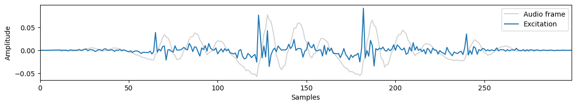
1. 对信号进行降采样（并预先进行低通滤波），使其采样频率为 10 kHz。

2. 通过线性预测技术对语音信号进行逆滤波，以获得声门波形。

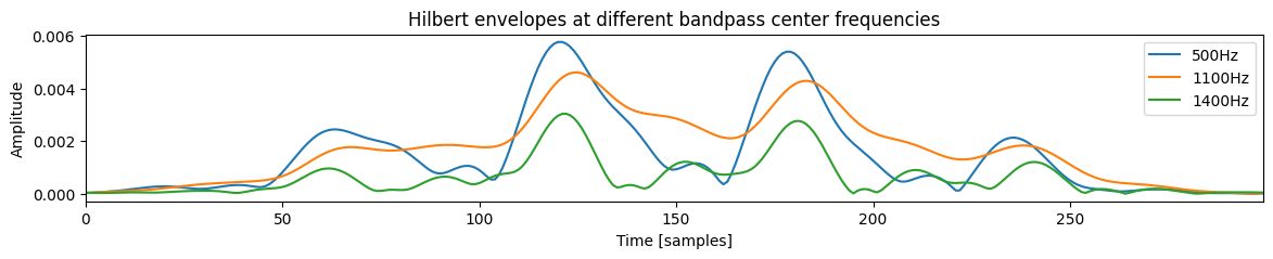
3. 对于每个窗口，计算具有固定带宽 (BW) 和不同中心频率的不同频带的希尔伯特包络。

4. 对于每个窗口，计算每对包络的互相关函数。

5. 将每对频带的互相关函数的最大值作为 GNE 分数。

# Step 1. Downsample to 10 kHz since voice energy is low above 5 kHz
new_sample_rate = 10000
downsampled_audio = torchaudio.functional.resample(audio, 44100, new_sample_rate)

# Step 2. Inverse filter with 30-msec window, 10-msec hop and 13th order LPC
frame_size, hop_size, lpc_order = 300, 100, 13

# Solve for LPC coefficients
window = torch.hann_window(frame_size).view(1, 1, -1)
gne_frames = downsampled_audio.view(1, -1).unfold(-1, frame_size, hop_size) * window

autocorrelation = compute_cross_correlation(gne_frames, gne_frames, width=lpc_order)

# Collapse frame and batch into same dimension, for lfiltering
batch, frame_count, _ = autocorrelation.shape
autocorrelation = autocorrelation.view(batch * frame_count, -1)

# Construct Toeplitz matrices (one per frame)
# This is [[p0, p1, p2...], [p1, p0, p1...], [p2, p1, p0...] ...]
# Our sliding window should go from the end to the front, so flip
# The autocorrelation has an extra value on each end for our prediction values
R = autocorrelation[:, 1: -1].unfold(-1, lpc_order, 1).flip(dims=(1,))
r = autocorrelation[:, lpc_order + 1:]

# Solve for LPC coefficients, generate inverse filter with coeffs 1, -a_1, ...
lpc = torch.linalg.solve(R, r)
a_coeffs = torch.cat((torch.ones(lpc.size(0), 1), -lpc), dim=1)
b_coeffs = torch.zeros_like(a_coeffs)
b_coeffs[:, 0] = 1

# Perform filtering
excitation = torchaudio.functional.lfilter(gne_frames, b_coeffs, a_coeffs, clamp=False)
plt.plot(gne_frames[0, 200, :] * 0.3, label='Audio frame', color="lightgrey")
plt.plot(excitation[0, 200, :], label='Excitation')
plt.xlabel("Samples")
plt.ylabel("Amplitude")
plt.legend()
plt.show()

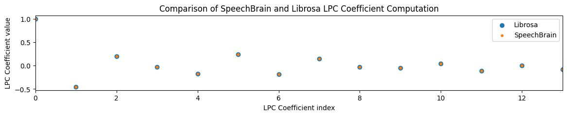
# Compare cf. librosa to check accuracy of LPC coefficients
import librosa

librosa_coeffs = librosa.lpc(gne_frames[0, 0].numpy(), order=lpc_order)
plt.scatter(torch.arange(lpc_order + 1), librosa_coeffs)
plt.scatter(torch.arange(lpc_order + 1), a_coeffs[0], s=10)
plt.legend(["Librosa", "SpeechBrain"])
plt.xlabel("LPC Coefficient index")
plt.ylabel("LPC Coefficient value")
plt.title("Comparison of SpeechBrain and Librosa LPC Coefficient Computation")
plt.show()

此处使用希尔伯特包络来估计声门脉冲串（在第 2 部分计算）在不同频带上的一致性。它的计算并非完全直接，你可以在此处看到一个示例

https://docs.scipy.org.cn/doc/scipy/reference/generated/scipy.signal.hilbert.html

虽然这些步骤隐藏在 compute_hilbert_envelopes() 调用中，但这些步骤（对于感兴趣的人）如下

(a) 对时域中的逆滤波语音信号应用实数离散时间傅里叶变换 (b) 在频域中选取每个频带并乘以一个 Hanning 窗 (c) 通过填充零（即，将负频率处的值设为零）使序列长度加倍 (d) 应用逆离散时间傅里叶变换 (e) 将获得的复数信号在时域中的绝对值作为希尔伯特包络。

步骤 b 到 e 应用于每个频带。

# Step 3. Compute Hilbert envelopes for each frequency bin
bandwidth = 1000
fshift = 300
min_freq, max_freq = bandwidth // 2, new_sample_rate // 2 - bandwidth // 2
center_freqs = range(min_freq, max_freq, fshift)
envelopes = {
    center_freq: compute_hilbert_envelopes(
        excitation, center_freq, bandwidth, new_sample_rate
    )
    for center_freq in center_freqs
}
plt.plot(envelopes[500][0, 200])
plt.plot(envelopes[1100][0, 200])
plt.plot(envelopes[1400][0, 200])
plt.legend(["500Hz", "1100Hz", "1400Hz"])
plt.title("Hilbert envelopes at different bandpass center frequencies")
plt.xlabel("Time [samples]")
plt.ylabel("Amplitude")
plt.show()

# Step 4. Compute cross correlation between (non-neighboring) frequency bins
correlations = [
    compute_cross_correlation(envelopes[freq_i], envelopes[freq_j], width=3)
    for freq_i in center_freqs
    for freq_j in center_freqs
    if (freq_j - freq_i) > bandwidth // 2
]

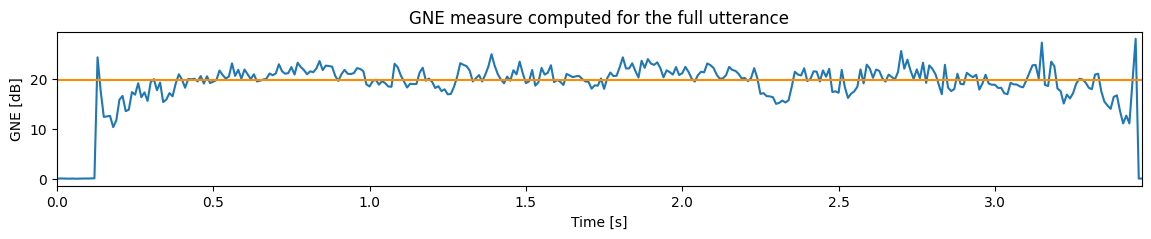
# Step 5. The maximum cross-correlation is the GNE score
gne = torch.stack(correlations, dim=-1).amax(dim=(2, 3))
gne = -10 * torch.log10(1 - gne)

new_step_size = hop_size / new_sample_rate
gne_xs = torch.arange(len(gne[0])) * new_step_size
plt.plot(gne_xs, gne[0])
plt.xlabel("Time [s]")
plt.ylabel("GNE [dB]")
plt.title("GNE measure computed for the full utterance")
plt.axhline(gne[gne > 10].mean(), color="darkorange")
print("Average GNE score:", gne[gne > 10].mean())

Average GNE score: tensor(19.8546)

PRAAT-Parselmouth

以下是与 PRAAT 的并行分析，以验证我们的度量看起来准确。为了在 Python 中计算 PRAAT 度量，我们使用 Parselmouth

• https://parselmouth.readthedocs.io/en/stable/

%%capture
!pip install praat-parselmouth

import parselmouth
from parselmouth.praat import call
import numpy as np

# Bundle these to compute them again later
def compute_praat_features(audio_filename):
    f0min = 75
    f0max = 300
    
    sound = parselmouth.Sound(audio_filename)
    pointProcess = call(sound, "To PointProcess (periodic, cc)", f0min, f0max)
    pitch = sound.to_pitch()
    pitch_values = pitch.selected_array['frequency']
    pitch_values[pitch_values==0] = np.nan

    jitter = call(pointProcess, "Get jitter (local)", 0, 0, 0.0001, 0.02, 1.3)
    shimmer = call([sound, pointProcess], "Get shimmer (local)", 0, 0, 0.0001, 0.02, 1.3, 1.6)

    harmonicity = sound.to_harmonicity()

    return pitch.xs() - 0.02, pitch_values, jitter, shimmer, harmonicity


pitch_xs, pitch_values, praat_jitter, praat_shimmer, praat_harmonicity = compute_praat_features(audio_filename)

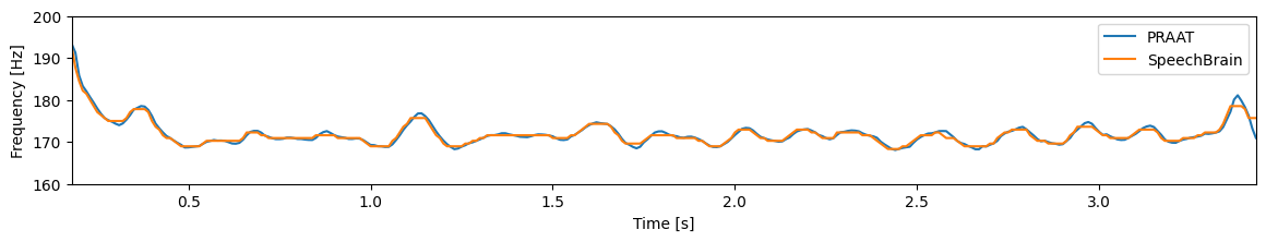
# Pitch comparison
plt.plot(pitch_xs, pitch_values)
voiced = np.isfinite(pitch_values[:-1])
plt.plot(xs[voiced], estimated_f0[0, voiced])
plt.ylim((160, 200))
plt.xlabel("Time [s]")
plt.ylabel("Frequency [Hz]")
plt.legend(["PRAAT", "SpeechBrain"])

print("Estimated average frequency (SpeechBrain): {0:.1f} Hz".format(estimated_f0[0, voiced].mean().numpy()))
print("Estimated average frequency (PRAAT): {0:.1f} Hz".format(np.nanmean(pitch_values)))

Estimated average frequency (SpeechBrain): 171.9 Hz
Estimated average frequency (PRAAT): 171.9 Hz

print("Average Jitter (SpeechBrain): {0:.2f}%".format(100 * jitter[0, voiced].mean().numpy()))
print("Average Jitter (PRAAT): {0:.2f}%".format(100 * praat_jitter))

Average Jitter (SpeechBrain): 0.50%
Average Jitter (PRAAT): 0.35%

print("Average Shimmer (SpeechBrain): {0:.2f}%".format(100 * shimmer[0, voiced].mean().numpy()))
print("Average Shimmer (PRAAT): {0:.2f}%".format(100 * praat_shimmer))

Average Shimmer (SpeechBrain): 2.40%
Average Shimmer (PRAAT): 2.25%

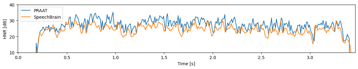
praat_hnr = call(praat_harmonicity, "Get mean", 0, 0)
plt.plot(praat_harmonicity.xs() - 0.02, praat_harmonicity.values.T)
plt.plot(xs[voiced], hnr[0, voiced])
plt.xlabel("Time [s]")
plt.ylabel("HNR [dB]")
plt.ylim((10, 40))
plt.legend(["PRAAT", "SpeechBrain"])
print("Average HNR (SpeechBrain): {0:.1f}%".format(hnr[0, voiced].mean().numpy()))
print("Average HNR (PRAAT): {0:.1f}%".format(praat_hnr))

Average HNR (SpeechBrain): 24.2%
Average HNR (PRAAT): 27.3%

与 OpenSMILE 比较

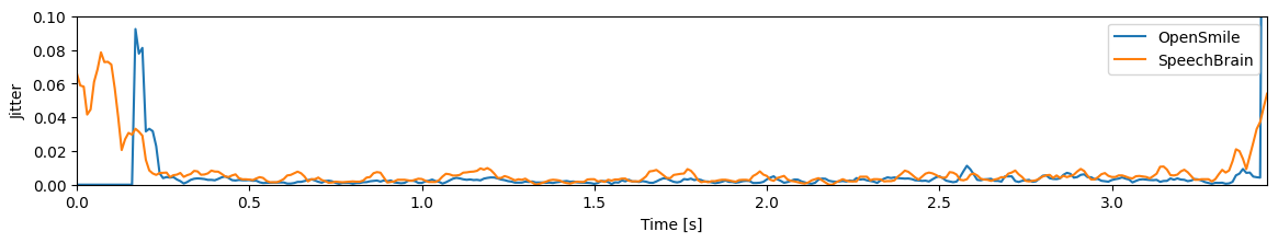
与 PRAAT 不同，我们可以使用 OpenSMILE 对 jitter 和 shimmer 进行逐帧比较，这有助于进一步验证我们的方法。

• https://www.audeering.com/opensmile/

%%capture
!pip install opensmile

import opensmile

opensmile_extractor = opensmile.Smile(
    feature_set=opensmile.FeatureSet.eGeMAPSv02,
    feature_level=opensmile.FeatureLevel.LowLevelDescriptors,
)

opensmile_feats = opensmile_extractor.process_file(audio_filename)
opensmile_feats.shape

(346, 25)

opensmile_feats.columns

Index(['Loudness_sma3', 'alphaRatio_sma3', 'hammarbergIndex_sma3',
       'slope0-500_sma3', 'slope500-1500_sma3', 'spectralFlux_sma3',
       'mfcc1_sma3', 'mfcc2_sma3', 'mfcc3_sma3', 'mfcc4_sma3',
       'F0semitoneFrom27.5Hz_sma3nz', 'jitterLocal_sma3nz',
       'shimmerLocaldB_sma3nz', 'HNRdBACF_sma3nz', 'logRelF0-H1-H2_sma3nz',
       'logRelF0-H1-A3_sma3nz', 'F1frequency_sma3nz', 'F1bandwidth_sma3nz',
       'F1amplitudeLogRelF0_sma3nz', 'F2frequency_sma3nz',
       'F2bandwidth_sma3nz', 'F2amplitudeLogRelF0_sma3nz',
       'F3frequency_sma3nz', 'F3bandwidth_sma3nz',
       'F3amplitudeLogRelF0_sma3nz'],
      dtype='object')

os_xs = opensmile_feats.index.get_level_values("start").total_seconds()
jitter_sma3 = torch.nn.functional.avg_pool1d(jitter, kernel_size=3, padding=1, stride=1, count_include_pad=False)
plt.plot(os_xs, opensmile_feats.jitterLocal_sma3nz)
plt.plot(xs, jitter_sma3[0])
plt.ylim((0, 0.1))
plt.xlabel("Time [s]")
plt.ylabel("Jitter")
plt.legend(["OpenSmile", "SpeechBrain"])
plt.show()

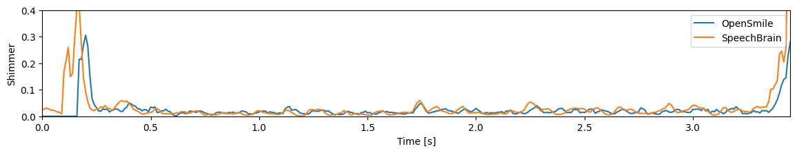
# From the name, it looks like shimmer should be in dB but the curve does not look it. Dividing by 10 is roughly the same.
plt.plot(os_xs, opensmile_feats.shimmerLocaldB_sma3nz / 10)
shimmer_sma3 = torch.nn.functional.avg_pool1d(shimmer, kernel_size=3, padding=1, stride=1, count_include_pad=False)
plt.plot(xs, shimmer_sma3[0])
plt.ylim((0, 0.4))
plt.xlabel("Time [s]")
plt.ylabel("Shimmer")
plt.legend(["OpenSmile", "SpeechBrain"])
plt.show()

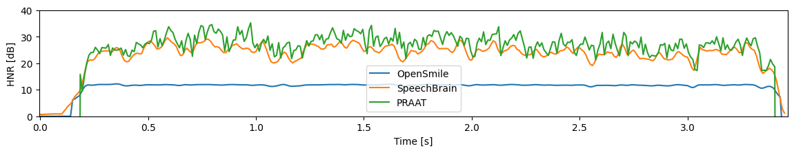
奇怪的是，OpenSmile 计算的 HNR（以 dB 为单位）似乎与 SpeechBrain 和 PRAAT 不匹配

plt.plot(os_xs, opensmile_feats.HNRdBACF_sma3nz)
hnr_sma3 = torch.nn.functional.avg_pool1d(hnr, kernel_size=3, padding=1, stride=1, count_include_pad=False)
plt.plot(xs, hnr_sma3[0])
plt.plot(praat_harmonicity.xs() - 0.02, praat_harmonicity.values.T)
plt.ylim(0, 40)
plt.xlabel("Time [s]")
plt.ylabel("HNR [dB]")
plt.legend(["OpenSmile", "SpeechBrain", "PRAAT"])
print("Maximum OpenSmile HNR value:", max(opensmile_feats.HNRdBACF_sma3nz))

Maximum OpenSmile HNR value: 12.219974517822266

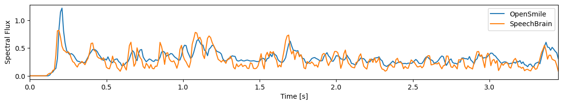
# Compute spectrum for remaining features
hann = torch.hann_window(window_samples).view(1, 1, -1)
spectrum = torch.abs(torch.fft.rfft(frames * hann))
spectral_feats = compute_spectral_features(spectrum)
# The last feature is flux
plt.plot(os_xs, opensmile_feats.spectralFlux_sma3)
plt.plot(xs, spectral_feats[0, :, -1])
plt.xlabel("Time [s]")
plt.ylabel("Spectral Flux")

plt.legend(["OpenSmile", "SpeechBrain"])
plt.show()

引用 SpeechBrain

如果你在研究或商业中使用了 SpeechBrain，请使用以下 BibTeX 条目引用它

@misc{speechbrainV1,
  title={Open-Source Conversational AI with {SpeechBrain} 1.0},
  author={Mirco Ravanelli and Titouan Parcollet and Adel Moumen and Sylvain de Langen and Cem Subakan and Peter Plantinga and Yingzhi Wang and Pooneh Mousavi and Luca Della Libera and Artem Ploujnikov and Francesco Paissan and Davide Borra and Salah Zaiem and Zeyu Zhao and Shucong Zhang and Georgios Karakasidis and Sung-Lin Yeh and Pierre Champion and Aku Rouhe and Rudolf Braun and Florian Mai and Juan Zuluaga-Gomez and Seyed Mahed Mousavi and Andreas Nautsch and Xuechen Liu and Sangeet Sagar and Jarod Duret and Salima Mdhaffar and Gaelle Laperriere and Mickael Rouvier and Renato De Mori and Yannick Esteve},
  year={2024},
  eprint={2407.00463},
  archivePrefix={arXiv},
  primaryClass={cs.LG},
  url={https://arxiv.org/abs/2407.00463},
}
@misc{speechbrain,
  title={{SpeechBrain}: A General-Purpose Speech Toolkit},
  author={Mirco Ravanelli and Titouan Parcollet and Peter Plantinga and Aku Rouhe and Samuele Cornell and Loren Lugosch and Cem Subakan and Nauman Dawalatabad and Abdelwahab Heba and Jianyuan Zhong and Ju-Chieh Chou and Sung-Lin Yeh and Szu-Wei Fu and Chien-Feng Liao and Elena Rastorgueva and François Grondin and William Aris and Hwidong Na and Yan Gao and Renato De Mori and Yoshua Bengio},
  year={2021},
  eprint={2106.04624},
  archivePrefix={arXiv},
  primaryClass={eess.AS},
  note={arXiv:2106.04624}
}