在 GitHub 上执行或查看/下载此笔记本

基于 Conformer 的流式语音识别

自动语音识别 (ASR) 模型通常只设计用于转录整个大块音频，不适用于需要低延迟、长篇转录的用例，如直播流转录。

本教程介绍了动态分块训练方法以及你可以应用的架构改动，以使 Conformer 模型具备流式能力。它介绍了 SpeechBrain 可以为你提供的训练和推理工具。如果你有兴趣训练和理解自己的流式模型，甚至想探索改进的流式架构，这可能是一个不错的起点。

本教程对实现细节进行了深入探讨。你可以根据自己的目标选择是否快速浏览。

此处描述的模型和训练过程并非最先进的，但它是一种相当不错且现代化的端到端方法。它已成功应用于以下 recipe (非详尽列表)

• LibriSpeech/ASR/transducer (在 HuggingFace 上预训练)

• VoxPopuli/ASR/transducer

• CommonVoice/ASR/transducer (法语、意大利语)

推荐的前置条件

• 从零开始的语音识别

安装 SpeechBrain

%%capture
# Installing SpeechBrain via pip
BRANCH = 'develop'
!python -m pip install git+https://github.com/speechbrain/speechbrain.git@$BRANCH

%%capture
%pip install matplotlib

流式模型需要实现的目标

我们需要一种细粒度的方式来限制和记忆上下文，以便模型只关注最近的上下文而非未来的帧。这种策略必须在训练和推理之间保持一致。

传统模型可能可以奢侈地在训练和推理时重用相同的前向代码路径。而流式模型的训练和推理具有相反的性能特征，这导致某些层需要特殊处理。

• 对于推理，我们通常需要随着输出的到来逐块处理，这通常意味着在不同层缓存一些过去的隐藏状态。

• 对于训练，我们倾向于一次性传入大量完整语句的批次，以最大化 GPU 利用率并降低 Python 和 CUDA 内核启动开销。因此，我们倾向于通过遮罩来强制执行这些限制。

教程总结

本教程尝试将理论和实践分成不同的章节。以下是各章节的总结：

1. 介绍 Conformer 模型的架构改动。我们将讨论：

   • 如何使用分块注意力遮罩解决自注意力机制的未来依赖问题。

   • 如何使用动态分块卷积解决卷积模块的未来依赖问题。

   • 为什么我们可以避免在训练时更改特征提取器和位置嵌入。

2. 解释动态分块训练策略。我们将讨论：

   • 如何训练模型以支持在运行时选择各种分块大小和左上下文大小。

   • 更改分块大小和左上下文大小的后果。

   • 不同损失函数对流式模型训练的影响。

3. 列出在 SpeechBrain 中训练流式 Conformer 所需的实际更改。

4. 解释如何调试神经网络层以确保正确的流式行为。

5. 介绍流式推理涉及的所有部分。我们将：

   • 介绍如何包装非流式特征提取器，使其成为流式提取器。

   • 解释流式上下文对象架构和流式前向方法。

   • 列出模型需要进行的其他杂项更改。

6. 实际介绍 SpeechBrain 中的推理工具。我们将：

   • 演示如何使训练好的流式模型准备好进行流式推理。

   • 提供 StreamingASR 推理接口用于流或文件处理的完整示例。

Conformer 架构的改动

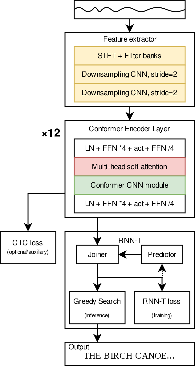
上图是我们某个模型中使用的普通 Conformer 架构的（非常）简化图，从上往下阅读。
彩色砖块是流式处理时需要我们特别小心的部分，因为它们在时间步长之间传播信息。

分块注意力

什么是因果注意力？

如果你熟悉 Transformer 架构，可能也熟悉因果注意力。简而言之，因果注意力使得时间步长 \(t\) 的输出帧无法关注来自“未来”时间步长（\(t+1\)、\(t+2\) 等）的输入。

这直接意味着，如果你想预测时间步长 \(t\) 的模型输出，你只需要“当前”和“过去”的输入（\(t\)、\(t-1\)、\(t-2\) 等）。这对我们很重要，因为我们不知道未来的帧！

因果注意力应用起来非常简单（朴素地），并且确实符合流式 ASR 的要求... 但我们在这里不使用它。

什么是分块注意力，为什么我们更喜欢它？

因果注意力实现简单，但在流式 ASR 中，发现它会显著降低词错误率。因此，流式注意力模型通常选择分块注意力。

从概念上讲，分块注意力引入了将给定数量帧 (chunk_size) 分组的块的概念。例如，如果你的块大小为 4，那么你将像这样查看输入：

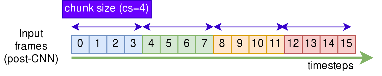
一个块内的帧可以互相关注。这与因果注意力相比，保留了注意力更多的表达能力。
块也可以关注过去的块，但我们限制了可以回溯多远，以减少推理时的计算和内存成本 (left_context_chunks)。

在训练时，我们使用注意力遮罩来强制执行这一点。注意力遮罩回答了这个问题：第 j 个输出帧可以关注第 i 个输入帧吗？
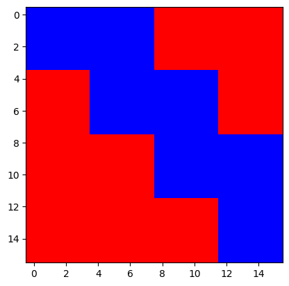
因此，它被定义为一个形状为 (t, t) 的布尔张量。下面是其中一个示例（尽管实际的遮罩是它的转置）：

事实上，我们可以相当容易地重现这个精确的遮罩。请注意，我们为了显示而转置了遮罩，并且在这里，True（红色）表示遮罩，False（蓝色）表示不遮罩。

from speechbrain.lobes.models.transformer.TransformerASR import make_transformer_src_mask
from speechbrain.utils.dynamic_chunk_training import DynChunkTrainConfig
from matplotlib import pyplot as plt
import torch

# dummy batch size, 16 sequence length, 128 sized embedding
chunk_streaming_mask = make_transformer_src_mask(torch.empty(1, 16, 128), dynchunktrain_config=DynChunkTrainConfig(4, 1))
plt.imshow(chunk_streaming_mask.T, cmap="bwr")
plt.show()

推理时的分块注意力

在设计流式模型时，我们需要非常小心输出帧和输入帧之间的依赖关系如何在层之间传播。

例如，回顾因果注意力，你可能会想，如果我们允许时间步长 \(t\) 的输出帧关注时间步长 \(t+1\) 的输入帧，即在每一层都为其提供一些“右侧”/未来上下文，是否能恢复一些准确性。
是的，我们可以，而且确实有点帮助，但考虑一下叠加层时的影响！例如，考虑两层注意力，其中 \(a\) 是输入，\(b\) 是第一层的输出，\(c\) 是第二层的输出：\(c_t\) 将关注 \(b_{t+1}\)（以及其他），而 \(b_{t+1}\) 本身将关注 \(a_{t+2}\)。在实际中，当可能有 12 或 17 层时，情况会变得更糟。
这很麻烦，并且可能会对延迟（我们需要缓冲大量“未来”帧）和内存/计算成本产生负面影响。

另一方面，分块注意力在这方面表现得非常好。让我们先忽略左上下文。 以下示例重点关注输入的第四个块，以及哪些帧实际依赖/关注哪些帧：

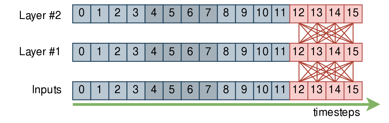
忽略左上下文，一个块内的帧可以互相关注。如果你叠加注意力层，块的边界在层之间保持不变。

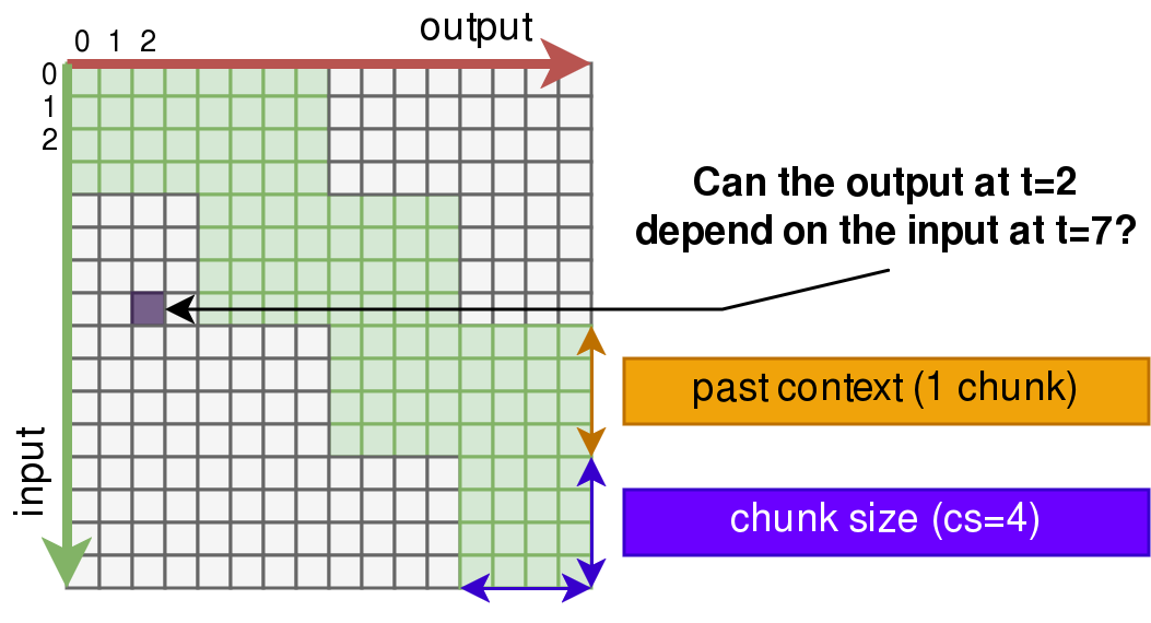
现在，让我们添加左上下文。在以下示例中，我们将假设左上下文大小为 1 个块。为清晰起见，我们省略了 12,13,14 的连接，但它们与 15 关注相同的帧。

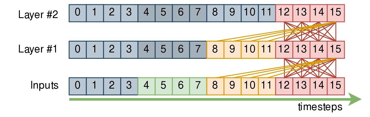
等等，这是否意味着 Layer #2 的输出 12,13,14,15 需要我们记住输入 4,5,6,7 的嵌入？

不！Layer #2 的 12,13,14,15 块确实依赖于 Layer #1 的 8,9,10,11，而后者本身依赖于 Inputs 的 4,5,6,7。
然而，Layer #1 中 8,9,10,11 的隐藏状态完全不受我们红色块的影响！因此，在推理时，我们可以缓存我们想使用的任意数量的左上下文块，并且需要缓存/重新计算的东西的数量不会随着层数的增加而爆炸。

speechbrain.lobes.models.transformer.TransformerASR.make_transformer_src_mask 是生成这些遮罩的函数。

在推理时这如何运作？

左上下文的定义是，给定块 \(i\) 可以关注 left_context_chunks 个块，即块 \(i\) 内的所有输出帧都可以关注过去 left_context_chunks 个块内的所有帧。
最终，这种设计使我们能够在推理时定义处理给定输入块注意力的数学，看起来像这样：

attention_module(concat(cached_left_chunks, input_chunk))

忽略 KV 缓存，此处，cached_left_chunks 最终将是每一层大小为 (batch_size, left_context_chunks * chunk_size, emb_dim) 的张量。这是相当合理的，也是我们在推理时对于注意力部分唯一需要保存的东西。

动态分块卷积

普通卷积

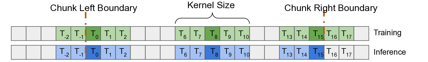
^{引用：Xilai Li 等，2023 年 (动态分块卷积论文)
卷积 \(k=5\) 的示例，意味着“半个窗口”，\(\frac{k-1}{2}\)，是 \(2\)。}

普通卷积在窗口上操作，对于时间步长 \(t\) 的卷积输出，窗口范围从 \(t-\frac{k-1}{2}\) 到 \(t+\frac{k-1}{2}\)，其中 \(k\) 是核大小。因此，时间步长 \(t\) 的输出将依赖于未来的帧，这是我们想要避免的。
我们可以假装忽略这个问题，正常训练，然后在推理时，将我们不知道的未来帧用零右填充（参见图）。然而，这将在训练和推理之间产生重大不匹配，并显著损害准确性。

因果卷积

存在一个直接的解决方案：因果卷积。它们仅仅将输出 \(t\) 的窗口移动，使其覆盖从 \(t-(k-1)\) 到 \(t\) 的索引。
计算方法非常简单：你只需要在输入左侧填充 \(\frac{k-1}{2}\) 帧，将其传递给卷积，并在左侧截断这 \(\frac{k-1}{2}\) 个输出帧。

动态分块卷积

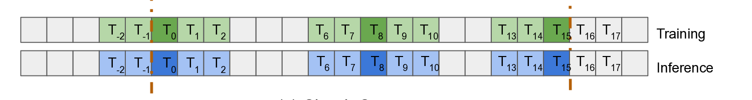
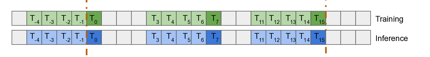
不幸的是，因果卷积会导致准确性下降。为了解决这个问题，Xilai Li 等，2023 年 提出了适用于流式分块 ASR 的动态分块卷积概念。

借此，我们重用了用于分块注意力的相同分块边界。
在上图中，考虑帧 \(T_{15}\)：它看起来很像普通卷积，除了属于未来块的任何输入帧都被遮罩掉了。这解决了我们依赖未来帧的问题。

注意示例块的最左侧输出 \(T_0\) 如何依赖于 \(\frac{k-1}{2}\) 个过去的帧：在推理时，我们需要在每一层缓存这一点。不过，这相对来说比较轻量级。

在训练时的实现实际上远非显而易见，因为 PyTorch 卷积算子不能像我们使用的自注意力遮罩那样简单地接受一个遮罩。如果你想冒险尝试，可以阅读 speechbrain.lobes.models.transformer.Conformer.ConvolutionModule 的源代码，其中包含了大量的（带有注释和图示的）张量重塑技巧。

我们没有改变什么

架构的某些部分并不真正重要，也不需要对流式处理进行特殊处理，因为它们不会在帧之间传播信息（即它们只是逐点操作）。
另一方面，有些部分需要一些解释，说明为什么它们重要或不重要。

特征提取

在 SpeechBrain 中实现时，Conformer 的特征提取器是非因果的。这通常是流式处理的一个问题，但我们在训练中保留了它。这是怎么回事？

事实证明，特征提取并不真正需要太多的右上下文（即看到许多未来帧）。我们可以负担得起为此引入一些右上下文的概念，因为它无论如何都代表着毫秒级的语音。这简化了整个过程，并为探索特征提取器提供了更大的灵活性。

SpeechBrain 提供了一个包装器 speechbrain.lobes.features.StreamingFeatureWrapper，它通过自动填充和缓存上下文，几乎完全为你抽象了这一点。它仍然需要被告知特征提取器的特性，我们稍后会详细介绍。

归一化是特征提取器的另一个未修改的部分。这实际上在训练和测试之间产生了差异，但我们发现它是最小的，即使在完整音频归一化和逐块归一化之间也是如此。因此，它几乎被忽略了，尽管你可以更仔细地处理它。

位置嵌入

我们在这里不会详细解释位置嵌入，尽管它们在 ASR 的模型准确性中起着重要作用。重要的是要知道它们用位置信息丰富了注意力机制。否则，模型将缺乏关于标记之间相对位置的信息。

幸运的是，我们正在使用在 SpeechBrain 中定义的使用相对位置正弦编码的模型 (speechbrain.nnet.attention.RelPosEncXL)。我们将在下面强调这为何有用。

在自注意力中，任何查询都可以关注任何键（只要该查询/键对未被遮罩，这对于分块注意力是必需的）。

• 如果没有位置嵌入，注意力机制将忽略查询和键在句子中的实际位置。

• 使用一个相当朴素的位置嵌入，我们会关注键相对于句子开头的位置。这可行，但对流式 ASR 在某些方面存在问题。最值得注意的是，距离会变得相当长。

• 使用我们的相对位置嵌入，我们查看查询和键之间的位置差值。

由于我们使用了分块注意力，它限制了查询可以关注过去和未来多远，因此我们编码的距离永远不会大于我们关注的帧窗口。
换句话说，如果我们使用 16 个 token 的块和 48 个 token 的左上下文进行关注，我们最多将表示从最右边的 token 到最左边的 token 的距离，即 \(63\)。
距离 \(63\) 将有其自己的固定位置编码向量，在自注意力中计算该特定查询/键对的分数时会考虑进去。

此外，无论我们在流中是 \(0\) 秒还是 \(30\) 分钟，这些距离都保持不变，因为它们是相对位置。

以下示例演示了在 16 个时间步长序列和 64 个嵌入大小上的相对位置编码：

from speechbrain.nnet.attention import RelPosEncXL
from matplotlib import pyplot as plt

test_pos_encoder = RelPosEncXL(64)
test_pos = test_pos_encoder.make_pe(seq_len=16)
print(f"(batch, seq_len*2-1, emb_size): {tuple(test_pos.shape)}")
plt.imshow(test_pos.squeeze(0).T, cmap="bwr")
plt.xlabel("seq_len*2-1")
plt.ylabel("emb_size")
plt.show()

(batch, seq_len*2-1, emb_size): (1, 31, 64)

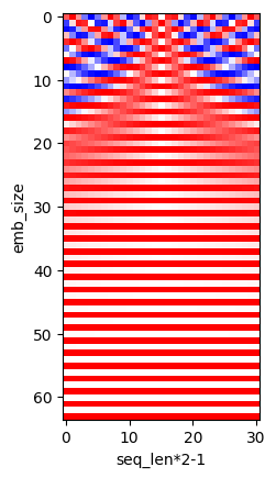
在上图中，中心列对应于位置差为零的位置嵌入向量，即，被关注的键与查询是相同的输入。

距离中心的水平距离代表自注意力内部给定查询和键对之间的距离。
中心右侧一列将代表距离 \(1\)，依此类推。

这不取决于键或查询与序列开头的距离。
在推理时，我们只需要使上面的 seq_len 达到注意力窗口的大小（左上下文 + 当前块）。

注意，这个嵌入首先通过一个可学习的线性层进一步丰富。

训练策略和动态分块训练

分块大小和左上下文大小影响哪些指标？

通常，在流式处理时，我们尝试以匹配分块大小的方式分割输入流，并随着块的到来逐个处理。

较小的块会更严重地降低准确性，但会带来较低的延迟。
这取决于最终的用例，是一种权衡，并且值得在代表最终应用程序的测试数据集上对不同的块大小进行基准测试。

查看 speechbrain/asr-streaming-conformer-librispeech 的数据，对于左块计数为 4 的情况，以及此特定模型和数据集，我们得到这样的曲线（请注意比例）：

from matplotlib import pyplot as plt
import matplotlib.ticker as mtick

xs = [1280,  960,  640,  480,  320]
ys = [3.10, 3.11, 3.31, 3.39, 3.62]
plt.scatter(xs, ys)
plt.plot(xs, ys)
plt.ylim(2, 4)
plt.title("asr-streaming-conformer-librispeech WER vs chunk size")
plt.xlabel("chunk size (ms)")
plt.ylabel("WER (%)")
plt.gca().yaxis.set_major_formatter(mtick.PercentFormatter())
plt.show()

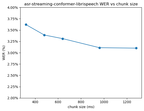
左上下文大小纯粹是准确性和计算/内存成本之间的权衡。在这里，也值得根据所需的权衡评估不同大小的模型。

如何选择分块大小？

奇怪的是，它不必是静态的！以下策略出人意料地有效：

• 对于 40% 的批次（随机选择），我们正常训练，不使用任何分块策略。

• 对于另外 60%，我们执行以下操作：

  • 对于每个批次，我们在一些合理的值之间采样一个随机的块大小（例如，在 8 到 32 个普通 conformer 帧之间进行均匀采样）。

  • 对于这些块中的 75%，我们类似地限制左上下文（例如，2-32 个块）。对于另外 25%，我们不限制。

这种策略在 SpeechBrain 中通过 speechbrain.utils.dynamic_chunk_training.DynChunkTrainConfigRandomSampler 进行抽象。

这样做的结果非常有趣：训练好的模型仍然可以以传统的非流式方式进行推理，但它也可以以在运行时选择的块大小进行流式推理！令人惊讶的是，我们发现在前一种情况下，相对于未修改的模型，错误率的下降有时是最小的，但对于其他超参数和数据集，影响可能会更显著。

让我们写一个例子

from speechbrain.core import Stage
from speechbrain.utils.dynamic_chunk_training import DynChunkTrainConfig
from speechbrain.utils.dynamic_chunk_training import DynChunkTrainConfigRandomSampler

sampler = DynChunkTrainConfigRandomSampler(
    chunkwise_prob=0.6,
    chunk_size_min=8,
    chunk_size_max=32,
    limited_left_context_prob=0.8,
    left_context_chunks_min=2,
    left_context_chunks_max=16,
    test_config=DynChunkTrainConfig(32, 16),
    valid_config=None
)

for i in range(10):
    print(f"Draw #{i:<2}     -> {sampler(Stage.TRAIN)}")

print()
print(f"Test config  -> {sampler(Stage.TEST)}")
print(f"Valid config -> {sampler(Stage.VALID)}")

Draw #0      -> None
Draw #1      -> DynChunkTrainConfig(chunk_size=5, left_context_size=None)
Draw #2      -> DynChunkTrainConfig(chunk_size=23, left_context_size=None)
Draw #3      -> None
Draw #4      -> DynChunkTrainConfig(chunk_size=12, left_context_size=14)
Draw #5      -> DynChunkTrainConfig(chunk_size=19, left_context_size=14)
Draw #6      -> DynChunkTrainConfig(chunk_size=24, left_context_size=None)
Draw #7      -> DynChunkTrainConfig(chunk_size=16, left_context_size=None)
Draw #8      -> DynChunkTrainConfig(chunk_size=8, left_context_size=6)
Draw #9      -> DynChunkTrainConfig(chunk_size=12, left_context_size=None)

Test config  -> DynChunkTrainConfig(chunk_size=32, left_context_size=16)
Valid config -> None

损失函数

目前训练流式 Conformer 模型最简单的方法是使用 RNN-T 损失（并可选地使用 CTC 作为辅助损失来改善训练）。为了回顾，请参阅从零开始的语音识别及其链接资源。

也可以将编码器-解码器交叉熵添加为辅助损失（即使使用 RNN-T 路径进行推理，也能提高模型准确性），或用于流式处理，但这尚未经过测试，目前也不受支持。
要实现这一点，你可能需要查阅文献并研究竞争性模型采用的方法。

训练：使用 SpeechBrain 将所有内容整合起来

讲了很多理论，但是我们如何利用 SpeechBrain 实现的功能呢？
以下描述了应该使用哪些代码，以及在典型的流式 Conformer-Transducer recipe 中有哪些流式专用代码。最好是改编一个已知的良好 recipe（例如 LibriSpeech/ASR/transducer）。

如果你正在尝试改编不同的模型，这可能会有所帮助，但你可能需要进行更多的研究和工作。

通过传递动态分块训练配置实现自动遮罩

添加了 speechbrain.utils.dynamic_chunk_training.DynChunkTrainConfig 类，其目的是描述一个批次的流式配置。为了实现完整的动态分块训练策略，你的训练脚本可以从 DynChunkTrainConfigRandomSampler 中为每个批次采样一个随机配置。（如果你愿意，可以自由实现自己的策略。）

各种函数得到了增强，例如 TransformerASR.encode，以接受 dynchunktrain_config 作为可选参数。
此参数允许你为这个特定的批次传递一个动态分块训练配置。当设置为 None 或未传递时，不会发生任何更改。

该参数会按需传递给每一层。使用标准的 Conformer 配置，传递此对象就是使编码器模块具备流式能力的全部所需。这使得浏览代码相当容易。

.yaml 文件中的改动

以下代码片段与此相关：

streaming: True  # controls all Dynamic Chunk Training & chunk size & left context mechanisms

正如前面所述，配置采样器对于在超参数中描述训练策略非常有用：

# Configuration for Dynamic Chunk Training.
# In this model, a chunk is roughly equivalent to 40ms of audio.
dynchunktrain_config_sampler: !new:speechbrain.utils.dynamic_chunk_training.DynChunkTrainConfigRandomSampler # yamllint disable-line rule:line-length
   chunkwise_prob: 0.6 # Probability during a batch to limit attention and sample a random chunk size in the following range
   chunk_size_min: 8 # Minimum chunk size (if in a DynChunkTrain batch)
   chunk_size_max: 32 # Maximum chunk size (if in a DynChunkTrain batch)
   limited_left_context_prob: 0.75 # If in a DynChunkTrain batch, the probability during a batch to restrict left context to a random number of chunks
   left_context_chunks_min: 2 # Minimum left context size (in # of chunks)
   left_context_chunks_max: 32 # Maximum left context size (in # of chunks)
   # If you specify a valid/test config, you can optionally have evaluation be
   # done with a specific DynChunkTrain configuration.
   # valid_config: !new:speechbrain.utils.dynamic_chunk_training.DynChunkTrainConfig
   #    chunk_size: 24
   #    left_context_size: 16
   # test_config: ...

确保你使用的是支持的架构（例如 Conformer，并且 TransformerASR 的 causal 参数设置为 False）。

目前，流式环境下只支持贪婪搜索。你可能希望将你的 test 集评估设置为使用贪婪搜索。

此外，你可以为采样器指定 valid_config 或 test_config（参见注释），以便在任一数据集上评估模型时模拟流式处理。

train.py 文件中的改动

在 compute_forward 中，你应该采样一个随机配置（以便每个批次都不同）：

if self.hparams.streaming:
    dynchunktrain_config = self.hparams.dynchunktrain_config_sampler(stage)
else:
    dynchunktrain_config = None

然后，假设编码器作为 enc 超参数可用，修改其调用以转发 dynchunktrain_config：

x = self.modules.enc(
    src,
    #...
    dynchunktrain_config=dynchunktrain_config,
)

对于训练，就这些了！

调试流式架构

speechbrain.utils.streaming 提供了一些有用的功能，包括我们将演示的调试特性。

检测神经网络层中的未来依赖项

你可能已经注意到，为现有架构添加流式支持并非易事，并且很容易忽略对未来的意外依赖。
speechbrain.utils.streaming.infer_dependency_matrix 可以为你计算输出帧和输入帧之间的依赖矩阵。
它通过重复调用你的模块，并找出哪些输出受到了哪些输入随机化的影响来实现这一点。
它还可以检测你的模型是否不够确定性，即连续两次调用产生了不同的数据。

然后可以使用 speechbrain.utils.streaming.plot_dependency_matrix 对输出进行可视化。
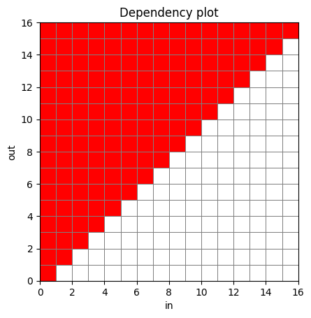
红色单元格表示给定输出的值可能受到给定输入的影响。因此，如果你看过前面的图，这些图可能会非常熟悉。
请注意，由于实现原因，在较大的图中和某些模型上，你可能会看到一些随机的空洞。这可能是假阴性。不要完全依赖 infer_dependency_matrix 来获得完美输出！

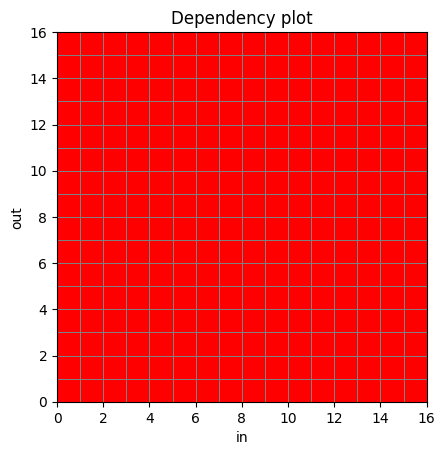
以下是实际 Conformer 层的依赖关系图示例：

from speechbrain.lobes.models.transformer.TransformerASR import TransformerASR
from speechbrain.utils.streaming import infer_dependency_matrix, plot_dependency_matrix
from matplotlib import pyplot as plt

noncausal_model = TransformerASR(
    tgt_vocab=64, input_size=64, d_model=64, nhead=1, d_ffn=64, 
    encoder_module="conformer", normalize_before=True,
    attention_type="RelPosMHAXL",
    num_encoder_layers=4, num_decoder_layers=0,
    causal=False
)
noncausal_model.eval()
noncausal_deps = infer_dependency_matrix(noncausal_model.encode, seq_shape=[1, 16, 64])
plot_dependency_matrix(noncausal_deps)
plt.show()

causal_model = TransformerASR(
    tgt_vocab=64, input_size=64, d_model=64, nhead=1, d_ffn=64, 
    encoder_module="conformer", normalize_before=True,
    attention_type="RelPosMHAXL",
    num_encoder_layers=4, num_decoder_layers=0,
    causal=True
)
causal_model.eval()
causal_deps = infer_dependency_matrix(causal_model.encode, seq_shape=[1, 16, 64])
plot_dependency_matrix(causal_deps)
plt.show()

from speechbrain.utils.dynamic_chunk_training import DynChunkTrainConfig

chunked_model = TransformerASR(
    tgt_vocab=64, input_size=64, d_model=64, nhead=1, d_ffn=64, 
    encoder_module="conformer", normalize_before=True,
    attention_type="RelPosMHAXL",
    num_encoder_layers=4, num_decoder_layers=0,
    causal=False
)
chunked_model.eval()
chunked_conf = DynChunkTrainConfig(chunk_size=4, left_context_size=1)
chunked_deps = infer_dependency_matrix(lambda x: chunked_model.encode(x, dynchunktrain_config = chunked_conf), seq_shape=[1, 16, 64])
plot_dependency_matrix(chunked_deps)
plt.show()

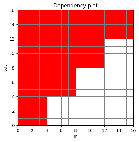
提醒一下，对于上面的图，例如时间步长 \(t=15\) 的输出依赖于 \(t=0\) 是正常的。
在任何一层中，\(t=15\) 都不直接关注 \(t=0\)。更多细节请阅读分块注意力部分。

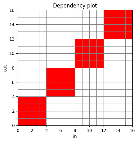
如果我们想看到纯粹的分块而不包含任何左上下文，我们可以减小卷积模块的核大小，完全禁用左上下文，然后观察到以下结果：

from speechbrain.utils.dynamic_chunk_training import DynChunkTrainConfig

chunked_model_nopast = TransformerASR(
    tgt_vocab=64, input_size=64, d_model=64, nhead=1, d_ffn=64, 
    encoder_module="conformer", normalize_before=True,
    attention_type="RelPosMHAXL",
    num_encoder_layers=4, num_decoder_layers=0,
    kernel_size=1,
    causal=False
)
chunked_model_nopast.eval()
chunked_conf = DynChunkTrainConfig(chunk_size=4, left_context_size=0)
chunked_deps = infer_dependency_matrix(lambda x: chunked_model_nopast.encode(x, dynchunktrain_config = chunked_conf), seq_shape=[1, 16, 64])
plot_dependency_matrix(chunked_deps)
plt.show()

推理：详细细节

为推理包装特征提取器

我们简要提到了为流式推理包装特征提取器。此处使用的 Conformer 特征提取器主要有三层：

1. 滤波器组提取，直接源自信号的傅里叶变换（参见傅里叶变换和谱图以及语音特征教程）。

2. 归一化（我们选择在流式处理时按块应用，如前所述——它并不真正影响结果）。

3. 两个下采样 CNN，每个都是步长为 2 的卷积，有效地将时间维度缩小 4 倍。

我们这里有两个问题：

• 我们在 Transformer 级别（特征提取后）定义块大小。因此，我们需要确切知道应该给提取器多少帧才能得到预期的形状。为此，我们需要确切知道特征提取器如何转换形状。

• 我们需要正确处理左/过去和右/未来上下文，以使特征提取器在行为上与训练时基本完全一致。

让我们尝试可视化这个问题。我们将定义一个相当标准的 Conformer 特征提取器用于 16kHz 输入波形。请注意，x 轴上的步长是 16，意味着 1ms。因此，x 轴计数可以看作毫秒（实际上输入样本比图中显示的多了 16 倍）。

from speechbrain.utils.streaming import infer_dependency_matrix, plot_dependency_matrix
from hyperpyyaml import load_hyperpyyaml
from matplotlib import pyplot as plt

feat_extractor_hparams = load_hyperpyyaml("""
compute_features: !new:speechbrain.lobes.features.Fbank
   sample_rate: 16000
   n_fft: 512
   n_mels: 80
   win_length: 32

cnn: !new:speechbrain.lobes.models.convolution.ConvolutionFrontEnd
   input_shape: (8, 10, 80)
   num_blocks: 2
   num_layers_per_block: 1
   out_channels: (64, 32)
   kernel_sizes: (3, 3)
   strides: (2, 2)
   residuals: (False, False)

feat_extractor: !new:speechbrain.nnet.containers.LengthsCapableSequential
    - !ref <compute_features>
    - !ref <cnn>

properties: !apply:speechbrain.utils.filter_analysis.stack_filter_properties
    - [!ref <compute_features>, !ref <cnn>]
""")
feat_extractor_hparams["cnn"].eval()

feat_extractor_deps = infer_dependency_matrix(
    # we need some shape magic here to adapt the input and output shape to what infer_dependency_matrix expects
    # for the input, squeeze the feature dimension
    # for the output, flatten the channels dim as the output is of shape [batch, t, c0, c1]
    lambda x: feat_extractor_hparams["feat_extractor"](x.squeeze(-1)).flatten(2),
    # 100ms audio (@16kHz)
    seq_shape=[1, 3200, 1],
    # 1ms stride (@16kHz)
    in_stride=16
)
feat_extractor_fig = plot_dependency_matrix(feat_extractor_deps)
feat_extractor_fig.set_size_inches(15, 10)
plt.show()

使用和定义滤波器属性

为了解决这个问题：

1. 我们将滤波器组提取和 CNN 视为具有特定步长、核大小（加上此处未使用的膨胀和因果性）的滤波器（在信号处理意义上）。在 SpeechBrain 中，这些数据表示为 FilterProperties。

2. 我们为某些模块提供了 get_filter_properties 方法（请注意，目前并非所有模块都有）。

3. 然后使用 stack_filter_properties 来“堆叠”这些滤波器，并获取整个特征提取器的最终属性。

让我们演示一下。

from speechbrain.utils.filter_analysis import stack_filter_properties

print(f"""Filter properties of the fbank module (including the STFT):
    fbank -> {feat_extractor_hparams['compute_features'].get_filter_properties()}

Filter properties of the downsampling CNN:
    ... of each layer:
    cnn[0] -> {feat_extractor_hparams['cnn']['convblock_0'].get_filter_properties()}
    cnn[1] -> {feat_extractor_hparams['cnn']['convblock_1'].get_filter_properties()}

    ... with both layers stacked:
    cnn    -> {feat_extractor_hparams['cnn'].get_filter_properties()}

Properties of the whole extraction module (fbank+CNN stacked):
    both   -> {feat_extractor_hparams['properties']}""")

Filter properties of the fbank module (including the STFT):
    fbank -> FilterProperties(window_size=512, stride=160, dilation=1, causal=False)

Filter properties of the downsampling CNN:
    ... of each layer:
    cnn[0] -> FilterProperties(window_size=3, stride=2, dilation=1, causal=False)
    cnn[1] -> FilterProperties(window_size=3, stride=2, dilation=1, causal=False)

    ... with both layers stacked:
    cnn    -> FilterProperties(window_size=7, stride=4, dilation=1, causal=False)

Properties of the whole extraction module (fbank+CNN stacked):
    both   -> FilterProperties(window_size=1473, stride=640, dilation=1, causal=False)

提取模块的步长是 640 个输入帧。由于我们处理的是 16kHz，这相当于一个有效步长约为 640/16000=40ms。
因此，一个块大小为 16 基本上意味着我们将在每个块中将输入移动 16*40ms=640ms，而无需担心窗口大小和填充。
请注意，这里的步长计算相对直观。你可能会注意到它是所有三个步长的乘积。窗口大小稍微复杂一些，完整的实现请参见 FilterProperties.with_on_top。

最终结果是，我们可以将特征提取器视为具有已知属性的简单滤波器。这解决了我们之前的两个问题，因为我们都知道：

• 特征提取器产生 chunk_size 个时间步长（在 Transformer 级别）所需的输入帧数。

• 窗口大小（以及其他属性），它使我们能够确切知道需要保留多少帧作为左和右上下文。

  • 重要提示： 特征提取器的有效窗口大小直接对延迟产生负面影响！窗口大小绝不能太大，接近块大小（以输入帧为单位）。

自动包装非流式提取器

StreamingFeatureWrapper 是特征提取难题的最后一块，它将我们有些任意的特征提取器转化为纯粹的块式提取器，后者接收固定且已知数量的输入帧（参见 StreamingFeatureWrapper.forward）。
如果你好奇，这是一个低级别的演示用法；否则，这完全由 StreamingASR 抽象。

from speechbrain.lobes.features import StreamingFeatureWrapper
from speechbrain.utils.dynamic_chunk_training import DynChunkTrainConfig

feature_wrapper = StreamingFeatureWrapper(
    module=feat_extractor_hparams["feat_extractor"],
    properties=feat_extractor_hparams["properties"]
)

filter_properties = feat_extractor_hparams["properties"]
chunk_size = 4
# see: StreamingFeatureWrapper.forward docs
# reason for the `-1` is that the stride is only applied `window_size-1` times in such a filter
chunk_size_frames = (filter_properties.stride - 1) * chunk_size
batch_size = 1

# a fair amount of streaming stuff carries around _streaming contexts_, which are opaque objects
# that you are meant to reuse across calls for the same streaming session.
# these will be detailed further in the next subsection.
streaming_context = feature_wrapper.make_streaming_context()

print(f"Chunk size selected: {chunk_size} ({chunk_size_frames} frames, {1000*chunk_size_frames/16000:.3f}ms)")

for t in range(4):  # imagine we're iterating over a stream, etc.
    sample_chunk = torch.rand((batch_size, chunk_size_frames))
    latest_outs = feature_wrapper(sample_chunk, context=streaming_context)
    print(f"(bs, t, ch0, ch1) = {tuple(latest_outs.shape)}")  # output for our chunk!

# normally you _may_ have to inject a final chunk of zeros.
# see StreamingASR for an example implementation.

Chunk size selected: 4 (2556 frames, 159.750ms)
(bs, t, ch0, ch1) = (1, 4, 20, 32)
(bs, t, ch0, ch1) = (1, 4, 20, 32)
(bs, t, ch0, ch1) = (1, 4, 20, 32)
(bs, t, ch0, ch1) = (1, 4, 20, 32)

这并没有告诉我们它到底做了什么。StreamingFeatureWrapper.forward 的源代码 真正最好地说明了这一点：

feat_pad_size = self.get_required_padding()
num_outputs_per_pad = self.get_output_count_per_pad_frame()

# consider two audio chunks of 6 samples (for the example), where
# each sample is denoted by 1, 2, ..., 6
# so chunk 1 is 123456 and chunk 2 is 123456
if context.left_context is None:
    # for the first chunk we left pad the input by two padding's worth of zeros,
    # and truncate the right, so that we can pretend to have right padding and
    # still consume the same amount of samples every time
    #
    # our first processed chunk will look like:
    # 0000123456
    #         ^^ right padding (truncated)
    #   ^^^^^^ frames that some outputs are centered on
    # ^^ left padding (truncated)
    chunk = torch.nn.functional.pad(chunk, (feat_pad_size * 2, 0))
else:
    # prepend left context
    #
    # for the second chunk ownwards, given the above example:
    # 34 of the previous chunk becomes left padding
    # 56 of the previous chunk becomes the first frames of this chunk
    # thus on the second iteration (and onwards) it will look like:
    # 3456123456
    #         ^^ right padding (truncated)
    #   ^^^^^^ frames that some outputs are centered on
    # ^^ left padding (truncated)
    chunk = torch.cat((context.left_context, chunk), 1)

# our chunk's right context will become the start of the "next processed chunk"
# plus we need left padding for that one, so make it double
context.left_context = chunk[:, -feat_pad_size * 2 :]

feats = self.module(chunk, *extra_args, **extra_kwargs)

# truncate left and right context
feats = feats[:, num_outputs_per_pad:-num_outputs_per_pad, ...]

return feats

在上面的例子中，我们实际上引入了 >80ms 的填充/延迟，如下所示：

print(f"{1000 * feature_wrapper.get_required_padding() / 16000}ms")

80.0ms

这并不理想，但对于通常在 500-1000ms 量级的块大小来说，这并不是一个巨大的惩罚。
然而，它确实强调了，虽然你可以调整特征提取器，但应该小心其有效窗口大小不要剧增。

流式上下文对象

为了实现流式处理，我们需要缓存/存储任意的上下文张量，以便在后续的块中重用。

由于这些对象与模型高度相关，并且功能很少共享，因此它们被实现为以下形式的数据类：

• 可变：上下文对象在给定块的前向传播后会更新。处理下一个块时应再次传递相同的对象。

• 递归：一个上下文对象可能包含任意数量的上下文对象。

• 不透明：这些包含的上下文对象可以是任意其他上下文对象类型，被视为需要在其间传递的黑箱。

每个这样的对象都包含任何所需的配置和一批流式会话。该对象将在调用它的任何层的后续调用中重复使用。

示例

我们的 Conformer 编码器的顶级类是 TransformerASR 抽象。

TransformerASRStreamingContext 是其相关的“流式上下文”。它定义为：

@dataclass
class TransformerASRStreamingContext:
    """Streaming metadata and state for a `TransformerASR` instance."""

    dynchunktrain_config: DynChunkTrainConfig
    """Dynamic Chunk Training configuration holding chunk size and context size
    information."""

    encoder_context: Any
    """Opaque encoder context information. It is constructed by the encoder's
    `make_streaming_context` method and is passed to the encoder when using
    `encode_streaming`.
    """

在上面的例子中，encoder_context 是一个任意类型的字段，取决于选择的具体编码器。
TransformerASR 不需要知道其细节；它只需要能够创建、存储并传递它（例如 TransformerASR.encode_streaming 将调用 encoder.forward_streaming 并传递 context=context.encoder_context）。

对于 Conformer，这将是一个 ConformerEncoderStreamingContext，它需要持有一个 ConformerEncoderLayerStreamingContext 列表（文档已精简）：

@dataclass
class ConformerEncoderStreamingContext:
    dynchunktrain_config: DynChunkTrainConfig
    layers: List[ConformerEncoderLayerStreamingContext]

ConformerEncoderLayerStreamingContext 本身需要存储一堆张量（文档已精简）：

@dataclass
class ConformerEncoderLayerStreamingContext:
    mha_left_context_size: int
    mha_left_context: Optional[torch.Tensor] = None
    dcconv_left_context: Optional[torch.Tensor] = None

因此，如果你有一个为 Conformer 配置的 TransformerASRStreamingContext 对象，你可以通过 context.encoder_context.layers[0].mha_left_context 访问第一层的 mha_left_context 缓存对象。

创建流式上下文对象

正如每个模块都有相应的 StreamingContext 数据类一样，它们也应该指定一个 make_streaming_context 方法。这会由父模块或用户调用。通常，它会接受一个 DynChunkTrainConfig 对象，但也有一些例外情况。
正如上下文的数据结构是任意递归的一样，make_streaming_context 可能会调用子模块自己的 make_streaming_context 方法。

让我们通过重用之前初始化的 TransformerASR 来演示：

test_context = chunked_model.make_streaming_context(DynChunkTrainConfig(16, 2))
test_context

TransformerASRStreamingContext(dynchunktrain_config=DynChunkTrainConfig(chunk_size=16, left_context_size=2), encoder_context=ConformerEncoderStreamingContext(dynchunktrain_config=DynChunkTrainConfig(chunk_size=16, left_context_size=2), layers=[ConformerEncoderLayerStreamingContext(mha_left_context_size=32, mha_left_context=None, dcconv_left_context=None), ConformerEncoderLayerStreamingContext(mha_left_context_size=32, mha_left_context=None, dcconv_left_context=None), ConformerEncoderLayerStreamingContext(mha_left_context_size=32, mha_left_context=None, dcconv_left_context=None), ConformerEncoderLayerStreamingContext(mha_left_context_size=32, mha_left_context=None, dcconv_left_context=None)]))

流式前向方法

对于需要流式上下文的模块，流式推理需要使用与通常的 forward 不同的方法，通常是 forward_streaming（但并非必需，例如参见 TransformerASR.encode_streaming）。

请参阅以下实际示例。在这里，我们选择块大小为 16，左上下文大小为 4 个块。请观察，对于每个后续块，左上下文张量的大小随着左上下文的到来而增加。一旦累积了足够的块，左上下文张量的大小就会保持在该长度。

test_context = chunked_model.make_streaming_context(DynChunkTrainConfig(16, 4))
for chunk_id in range(8):
    print(f"chunk #{chunk_id}:")
    test_chunk = torch.rand((1, 16, 64))
    test_mha_context = test_context.encoder_context.layers[0].mha_left_context
    model_output = chunked_model.encode_streaming(test_chunk, context=test_context)
    
    print(f"\tbefore forward MHA left context: {tuple(test_mha_context.shape) if test_mha_context is not None else '(None)'}")
    print(f"\tencode_streaming output:         {tuple(model_output.shape)}")

chunk #0:
	before forward MHA left context: (None)
	encode_streaming output:         (1, 16, 64)
chunk #1:
	before forward MHA left context: (1, 16, 64)
	encode_streaming output:         (1, 16, 64)
chunk #2:
	before forward MHA left context: (1, 32, 64)
	encode_streaming output:         (1, 16, 64)
chunk #3:
	before forward MHA left context: (1, 48, 64)
	encode_streaming output:         (1, 16, 64)
chunk #4:
	before forward MHA left context: (1, 64, 64)
	encode_streaming output:         (1, 16, 64)
chunk #5:
	before forward MHA left context: (1, 64, 64)
	encode_streaming output:         (1, 16, 64)
chunk #6:
	before forward MHA left context: (1, 64, 64)
	encode_streaming output:         (1, 16, 64)
chunk #7:
	before forward MHA left context: (1, 64, 64)
	encode_streaming output:         (1, 16, 64)

流式分词器

尽管如此，我们仍然需要关注流式环境下的分词这个小细节。

通常，分词器总是一次性解码整个句子，因此解码中第一个空格（例如 are token 中的空格）会被移除。
然而，在流式处理时，我们可能正在解码句中，此时句中的空格不能被移除中句。spm_decode_preserve_leading_space 处理这种情况，并需要携带一个小的上下文对象。

流式 Transducer 贪婪搜索

TransducerBeamSearcher 提供了一个 transducer_greedy_decode_streaming 方法，与其他 _streaming 方法一样，它要求用户创建并携带一个上下文对象。

在这种情况下，它是一个相当简单的包装器，用于缓存和传递贪婪搜索器的最新隐藏状态。

推理：StreamingASR 的实际示例

从训练好的模型到 StreamingASR 超参数

目前，在 SpeechBrain 中，你需要为训练和推理分别定义超参数文件。你基本上可以复制训练超参数，并根据推理的需要删除/添加键。
在这种情况下，更高级别的推理接口 speechbrain.inference.ASR.StreamingASR 需要由推理超参数定义一组特定的键和模块，并且方式相对灵活。

如果你查看文档，你可以找到以下超参数键和 modules 字典条目要求：

HPARAMS_NEEDED = [
    "fea_streaming_extractor",
    "make_decoder_streaming_context",
    "decoding_function",
    "make_tokenizer_streaming_context",
    "tokenizer_decode_streaming",
]
MODULES_NEEDED = ["enc", "proj_enc"]

让我们看看这意味着什么。对于我们的 Conformer 模型，我们可以参考 speechbrain/asr-streaming-conformer-librispeech。（提醒一下，以 !name: 初始化的键在这里只是函数的引用。）请参阅：

make_tokenizer_streaming_context: !name:speechbrain.tokenizers.SentencePiece.SentencePieceDecoderStreamingContext
tokenizer_decode_streaming: !name:speechbrain.tokenizers.SentencePiece.spm_decode_preserve_leading_space

make_decoder_streaming_context: !name:speechbrain.decoders.transducer.TransducerGreedySearcherStreamingContext # default constructor
decoding_function: !name:speechbrain.decoders.transducer.TransducerBeamSearcher.transducer_greedy_decode_streaming
   - !ref <Greedysearcher>  # self

fea_streaming_extractor: !new:speechbrain.lobes.features.StreamingFeatureWrapper
   module: !new:speechbrain.nnet.containers.LengthsCapableSequential
      - !ref <compute_features>
      - !ref <normalize>
      - !ref <CNN>
   # don't consider normalization as part of the input filter chain.
   # normalization will operate at chunk level, which mismatches training
   # somewhat, but does not appear to result in noticeable degradation.
   properties: !apply:speechbrain.utils.filter_analysis.stack_filter_properties
      - [!ref <compute_features>, !ref <CNN>]

结合前面的细节，此处不应有特别令人惊讶之处。但是，更详细地说，其思想是通过超参数文件为模型提供一定的灵活性。我们实际上需要定义：

1. fea_streaming_extractor 是一个 StreamingFeatureWrapper（或任何具有兼容API的东西），它处理输入波形（同时提供滤波器属性等）

2. modules.enc 和 modules.proj_enc，实际的编码器，请参见 StreamingASR.encode_chunk 的源代码

3. decoding_function，可以像 hparams.decoding_function(output_of_enc, context=decoding_context) 这样调用，其中…

4. … decoding_context 从 hparams.make_decoder_streaming_context() 初始化

5. tokenizer_decode_streaming 和 make_decoder_streaming_context，请参见 StreamingASR.decode_chunk 的源代码

至于训练后需要从保存目录移动到典型的 `StreamingASR` 流式 Conformer 模型目录的文件，它们基本上是

• hyperparams.yaml（为推理修改后）

• model.ckpt

• normalizer.ckpt

• tokenizer.ckpt

使用 StreamingASR 进行推理

让我们利用 speechbrain/asr-streaming-conformer-librispeech 来演示流式音频解码。

from speechbrain.inference.ASR import StreamingASR
from speechbrain.utils.dynamic_chunk_training import DynChunkTrainConfig
asr_model = StreamingASR.from_hparams("speechbrain/asr-streaming-conformer-librispeech")

INFO:speechbrain.utils.fetching:Fetch hyperparams.yaml: Fetching from HuggingFace Hub 'speechbrain/asr-streaming-conformer-librispeech' if not cached
INFO:speechbrain.utils.fetching:Fetch custom.py: Fetching from HuggingFace Hub 'speechbrain/asr-streaming-conformer-librispeech' if not cached
INFO:speechbrain.utils.fetching:Fetch model.ckpt: Fetching from HuggingFace Hub 'speechbrain/asr-streaming-conformer-librispeech' if not cached
INFO:speechbrain.utils.fetching:Fetch model.ckpt: Fetching from HuggingFace Hub 'speechbrain/asr-streaming-conformer-librispeech' if not cached
INFO:speechbrain.utils.fetching:Fetch normalizer.ckpt: Fetching from HuggingFace Hub 'speechbrain/asr-streaming-conformer-librispeech' if not cached
INFO:speechbrain.utils.fetching:Fetch normalizer.ckpt: Fetching from HuggingFace Hub 'speechbrain/asr-streaming-conformer-librispeech' if not cached
INFO:speechbrain.utils.fetching:Fetch tokenizer.ckpt: Fetching from HuggingFace Hub 'speechbrain/asr-streaming-conformer-librispeech' if not cached
INFO:speechbrain.utils.fetching:Fetch tokenizer.ckpt: Fetching from HuggingFace Hub 'speechbrain/asr-streaming-conformer-librispeech' if not cached
INFO:speechbrain.utils.parameter_transfer:Loading pretrained files for: model, normalizer, tokenizer

这是一个简单的转录示例，它*确实*执行分块推理

asr_model.transcribe_file(
    "speechbrain/asr-streaming-conformer-librispeech/test-en.wav",
    # select a chunk size of ~960ms with 4 chunks of left context
    DynChunkTrainConfig(24, 4),
    # disable torchaudio streaming to allow fetching from HuggingFace
    # set this to True for your own files or streams to allow for streaming file decoding
    use_torchaudio_streaming=False,
)

INFO:speechbrain.utils.fetching:Fetch test-en.wav: Fetching from HuggingFace Hub 'speechbrain/asr-streaming-conformer-librispeech' if not cached

'THE BIRCH CANOE SLID ON THE SMOOTH PLANKS'

让我们尝试一个更具挑战性的示例：转录一个几分钟长的音频文件。由于 transformer 处理长序列时内存和计算成本较高，这通常会导致序列过长而无法处理。

这次，让我们使用 transcribe_file_streaming。这个方法使我们能够迭代处理已转录的块。

from speechbrain.utils.fetching import fetch

long_audio_fname = fetch("Economics-of-coffee.ogg", "https://upload.wikimedia.org/wikipedia/commons/8/81", savedir=".")
long_audio_chunks = []

for i, decoded_chunk in enumerate(asr_model.transcribe_file_streaming(long_audio_fname, DynChunkTrainConfig(16, 4))):
    print(f"{i:>3}: \"{decoded_chunk}\"")
    long_audio_chunks.append(decoded_chunk)

    # let's just process the 20 first chunks as a demo
    if i >= 20:
        break

INFO:speechbrain.utils.fetching:Fetch Economics-of-coffee.ogg: Using existing file/symlink in /home/sdelang/projects/src/python/speechbrain/docs/tutorials/nn/Economics-of-coffee.ogg

  0: ""
  1: ""
  2: "ECONOMICS"
  3: " OF COFFEE"
  4: ""
  5: " FROM"
  6: " WICKPEDIA"
  7: " THE FREE"
  8: " SECLOPAEDIA"
  9: ""
 10: ""
 11: " COFFEE"
 12: " IS AN IMPORTAN"
 13: "T COM"
 14: "MODITY"
 15: " AND A POPULAR"
 16: " BEVERAGE"
 17: ""
 18: " OVER A TWO POINT"
 19: " TWO FIVE BILL"
 20: "ION CUPS"

模型出现了一些错误（考虑到其训练数据和我们正在测试的推理方式，这并不特别令人惊讶），但除此之外，流式处理似乎工作正常，跨块的单词转录看起来也没有乱码。

ffmpeg 直播流功能

StreamingASR 支持 torchaudio 的 ffmpeg 流媒体功能。这意味着您可以轻松地做一些事情，比如转录网络电台流

audio_stream_url = "http://as-hls-ww-live.akamaized.net/pool_904/live/ww/bbc_radio_fourfm/bbc_radio_fourfm.isml/bbc_radio_fourfm-audio%3d96000.norewind.m3u8"

for i, decoded_chunk in enumerate(asr_model.transcribe_file_streaming(audio_stream_url, DynChunkTrainConfig(16, 4))):
    print(decoded_chunk, end="")

    # let's just process the 20 first chunks as a demo
    if i >= 20:
        break

THEY WERE SO QUICK THEY DID THIS AIM AND THEN IT TOOK THEM TWO DAYS TO INSTALL THE SECOND DAY THEY WORKED UNTIL AFTER SEVEN P M AND THAT WAS IT I MEAN YET LIKE

手动转录块

模型在 HuggingFace 页面上提供了更多示例。特别是，Gradio 示例展示了如何自己处理任意音频块流，绕过音频加载功能。

替代方案和进一步阅读

本教程涵盖了对大部分原生 Conformer 模型进行修改以支持分块流式处理。
多年来，已经开发了 Conformer 模型的替代方案和改进，以提高准确性、提高运行时性能、降低内存使用、降低实际延迟或添加其他功能。
以下远非完整列表，它不仅包括已成功适应流式处理环境的架构。

• Branchformer（和 E-Branchformer）

• Zipformer（由 k2/icefall 等实现，以及其他 Conformer 变体，已实现流式支持）

• FastConformer（尽管它很简单，但截至 2024 年仍被 NVIDIA 大量使用，并且易于从原生 Conformer 迁移）

围绕训练或推理管道的其他部分也有大量研究。未来我们可能会通过更多参考资料扩展此列表

• 剪枝 RNN-T

引用 SpeechBrain

如果您在研究或商业中使用 SpeechBrain，请使用以下 BibTeX 条目引用它

@misc{speechbrainV1,
  title={Open-Source Conversational AI with {SpeechBrain} 1.0},
  author={Mirco Ravanelli and Titouan Parcollet and Adel Moumen and Sylvain de Langen and Cem Subakan and Peter Plantinga and Yingzhi Wang and Pooneh Mousavi and Luca Della Libera and Artem Ploujnikov and Francesco Paissan and Davide Borra and Salah Zaiem and Zeyu Zhao and Shucong Zhang and Georgios Karakasidis and Sung-Lin Yeh and Pierre Champion and Aku Rouhe and Rudolf Braun and Florian Mai and Juan Zuluaga-Gomez and Seyed Mahed Mousavi and Andreas Nautsch and Xuechen Liu and Sangeet Sagar and Jarod Duret and Salima Mdhaffar and Gaelle Laperriere and Mickael Rouvier and Renato De Mori and Yannick Esteve},
  year={2024},
  eprint={2407.00463},
  archivePrefix={arXiv},
  primaryClass={cs.LG},
  url={https://arxiv.org/abs/2407.00463},
}
@misc{speechbrain,
  title={{SpeechBrain}: A General-Purpose Speech Toolkit},
  author={Mirco Ravanelli and Titouan Parcollet and Peter Plantinga and Aku Rouhe and Samuele Cornell and Loren Lugosch and Cem Subakan and Nauman Dawalatabad and Abdelwahab Heba and Jianyuan Zhong and Ju-Chieh Chou and Sung-Lin Yeh and Szu-Wei Fu and Chien-Feng Liao and Elena Rastorgueva and François Grondin and William Aris and Hwidong Na and Yan Gao and Renato De Mori and Yoshua Bengio},
  year={2021},
  eprint={2106.04624},
  archivePrefix={arXiv},
  primaryClass={eess.AS},
  note={arXiv:2106.04624}
}