在 GitHub 上执行或查看/下载此笔记本

语音增强

机器学习中有一句流行语是“数据越多越好”。然而，收集新数据成本可能很高，我们必须巧妙地利用现有数据集。

一种流行的技术称为语音增强。其思想是人为地损坏原始语音信号，给网络造成正在处理新信号的“错觉”。这是一种强大的正则化技术，通常有助于神经网络提高泛化能力并在测试数据上获得更好的性能。

SpeechBrain 目前支持多种增强技术

1. 速度扰动

2. 时间丢弃（分块丢弃）

3. 频率丢弃（频率丢弃）

4. 削波

5. 随机振幅

6. 通道丢弃（用于多通道数据）

7. 通道交换（用于多通道数据）

8. CutCat（用于多通道数据）

9. 降低位深

10. 添加噪声

11. 添加混响

最后两项在此处介绍。

本教程将介绍 speechbrain.augment 中实现的一些增强技术。让我们从安装 SpeechBrain 开始吧。

首先，让我们安装 SpeechBrain。

%%capture

# Installing SpeechBrain via pip
BRANCH = 'develop'
!python -m pip install git+https://github.com/speechbrain/speechbrain.git@$BRANCH

我们还下载一个语音信号用于测试

%%capture
!wget https://www.dropbox.com/s/u8qyvuyie2op286/spk1_snt1.wav

%matplotlib inline
%config InlineBackend.figure_format = "jpg"

1. 速度扰动

通过速度扰动，我们将音频信号重采样到与原始采样率略有不同的采样率。通过这个简单的技巧，我们可以合成听起来比原始信号“更快”或“更慢”的语音信号。请注意，这不仅影响语速，还影响说话人的音高和共振峰等特征。

现在让我们试试吧！

首先，让我们读取一个语音信号

import matplotlib.pyplot as plt
from speechbrain.dataio.dataio import read_audio
signal = read_audio('spk1_snt1.wav')
plt.figure(1)
plt.title("Original Speech")
plt.plot(signal)
plt.show()

您也可以播放音频

from IPython.display import Audio
Audio('spk1_snt1.wav')

现在我们可以初始化速度扰动器了

from speechbrain.augment.time_domain import SpeedPerturb

perturbator = SpeedPerturb(orig_freq=16000, speeds=[90])

速度扰动器是一个类，可以使用三个参数进行初始化

• orig_freq：它是原始信号的采样频率

• speeds：这是一个列表，包含信号应更改到的所有速度，以原始信号的百分比表示（例如，speed=[100] 不会更改原始信号）。当添加更多值时（例如，speed=[90, 100, 110, 120]），速度将从指定值中随机选择。

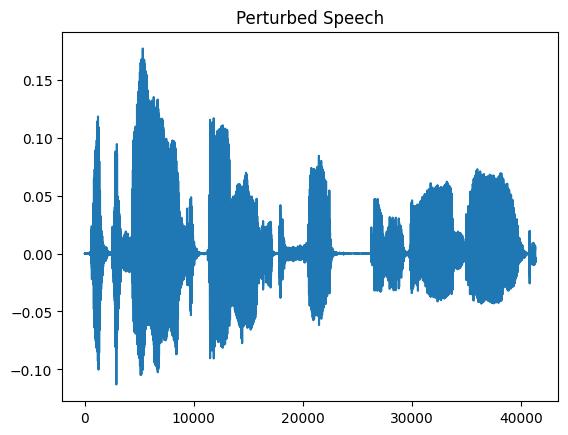
现在让我们将其应用于原始信号

clean = signal.unsqueeze(0) # [batch, time]
perturbed = perturbator(clean)

plt.figure(1)
plt.title("Perturbed Speech")
plt.plot(perturbed.squeeze())
plt.show()

print(clean.shape)
print(perturbed.shape)

Audio(perturbed,rate=16000)

torch.Size([1, 45920])
torch.Size([1, 41328])

扰动后的张量包含扰动后的语音信号。可以从原始信号与扰动后信号的形状（41328/45920 = 0.9）中看出，变化因子是 90%。

需要注意的另一件事是，此函数支持多个输入批量，并且必须对原始信号进行 unsqueeze 以在张量的第一个维度中分配批量维度。

2. 时间丢弃

分块丢弃将原始波形中的一些随机分块替换为零。其直觉是，即使信号的某些部分缺失，神经网络也应该提供良好的性能。从概念上讲，这类似于dropout。不同之处在于，它仅应用于输入波形。另一个区别是，我们丢弃的是连续样本，而不是像 dropout 那样随机选择的元素。

让我们看一个示例

import torch
from speechbrain.augment.time_domain import DropChunk

dropper = DropChunk(drop_length_low=2000, drop_length_high=3000, drop_count_low=5, drop_count_high=10)
length = torch.ones(1)
dropped_signal = dropper(clean, length)

plt.figure(1)
plt.title("Signal after Drop Chunk")
plt.plot(dropped_signal.squeeze())
plt.show()

Audio(dropped_signal,rate=16000)

在上面的示例中，我们略微夸大了效果，使其更明显。可以通过调整以下参数来控制零的数量

• drop_length_low 和 drop_length_high ，它们决定了随机零分块的最大和最小长度。

• drop_count_low 和 drop_count_high ，它们影响添加到原始信号中的随机分块数量

需要长度向量是因为我们可以并行处理长度不同的信号批量。长度向量包含构成批量的每个句子的相对长度（例如，对于两个批量，我们可以有 length=[0.8 1.0]，其中 1.0 是批量中最长句子的长度）。在这种情况下，我们有一个由单个句子组成的批量，因此相对长度是 length=[1.0]。

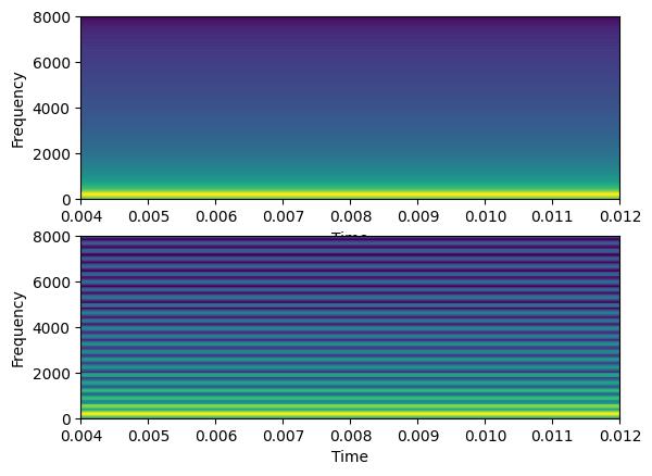
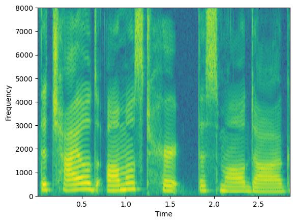
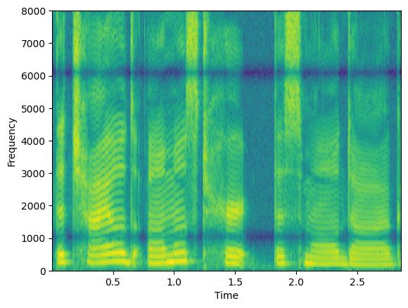
3. 频率丢弃

频率丢弃不是在时域中添加零，而是在频域中添加零。这可以通过使用随机选择的带阻滤波器过滤原始信号来实现。与分块丢弃类似，直觉是即使某些频率通道缺失，神经网络也应该能很好地工作。

from speechbrain.augment.time_domain import DropFreq

dropper = DropFreq(drop_freq_count_low=5, drop_freq_count_high=8)
dropped_signal = dropper(clean)

# Let's plot the two spectrograms
plt.subplot(211)
plt.specgram(clean.squeeze(),Fs=16000)
plt.xlabel('Time')
plt.ylabel('Frequency')

plt.subplot(212)
plt.specgram(dropped_signal.squeeze(),Fs=16000)
plt.xlabel('Time')
plt.ylabel('Frequency')

Text(0, 0.5, 'Frequency')

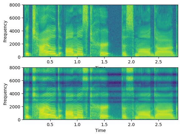
频率丢弃量由以下参数控制

• drop_count_low/drop_count_high，它们影响要丢弃的频带数量。

• drop_freq_low/drop_freq_high，它们对应于可以丢弃的最小和最大频率。

• drop_width，它对应于要丢弃的频带宽度。

4. 削波

另一种从语音信号中移除部分信息的方法是添加削波。它是一种非线性失真形式，它限制信号的最大绝对幅度（从而产生饱和效果）。

import torch
from speechbrain.augment.time_domain import DoClip

clipper = DoClip(clip_low=0.7, clip_high=0.7)
sinusoid = torch.sin(torch.linspace(0,20, 300))
clipped_signal = clipper(sinusoid.unsqueeze(0))

#  plots
plt.figure(1)
plt.subplot(211)
plt.plot(sinusoid)
plt.xlabel('Time')

plt.subplot(212)
plt.plot(clipped_signal.squeeze())
plt.xlabel('Time')

# freq domain
plt.figure(2)
plt.subplot(211)
plt.specgram(sinusoid,Fs=16000)
plt.xlabel('Time')
plt.ylabel('Frequency')

plt.subplot(212)
plt.specgram(clipped_signal.squeeze(),Fs=16000)
plt.xlabel('Time')
plt.ylabel('Frequency')

Text(0, 0.5, 'Frequency')

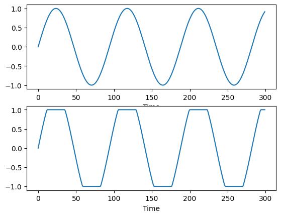
削波量由参数 clip_low 和 clip_high 控制，它们设置了信号被限制的下限和上限阈值。在频域中，削波在频谱的高频部分添加谐波。

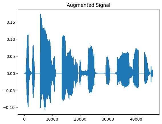
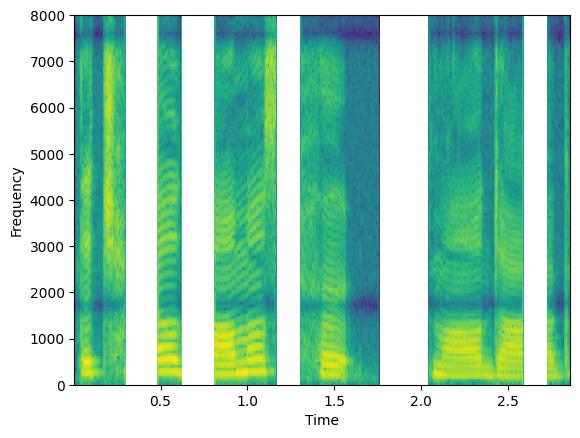
5. 增强组合

让我们考虑这样一个场景：您希望通过以随机方式整合先前定义的增强技术来构建增强管道。

这种集成由 speechbrain.augment 模块中一个名为 Augmenter 的专用类提供便利。

为简单起见，让我们看看一个想要结合频率丢弃器和分块丢弃器的情况

from speechbrain.augment.time_domain import DropFreq, DropChunk
from speechbrain.augment.augmenter import Augmenter

freq_dropper = DropFreq()
chunk_dropper = DropChunk(drop_length_low=2000, drop_length_high=3000, drop_count_low=5, drop_count_high=10)
augment = Augmenter(parallel_augment=False, concat_original=False, min_augmentations=2, max_augmentations=2,
                    shuffle_augmentations=False, repeat_augment=1,augmentations=[freq_dropper, chunk_dropper])

augmented_signal, lenghts = augment(clean, lengths=torch.tensor([1.0]))


plt.figure(1)
plt.title("Augmented Signal")
plt.plot(augmented_signal.squeeze())
plt.show()

plt.specgram(augmented_signal.squeeze(),Fs=16000)
plt.xlabel('Time')
plt.ylabel('Frequency')



Audio(augmented_signal,rate=16000)

/home/sdelang/env/sb312/lib/python3.12/site-packages/matplotlib/axes/_axes.py:8089: RuntimeWarning: divide by zero encountered in log10
  Z = 10. * np.log10(spec)

The Augmenter 通过 augmentations 参数接受增强技术，并将它们组合起来生成增强后的输出。

用户可以灵活设置各种超参数，根据自己的偏好定制增强策略。

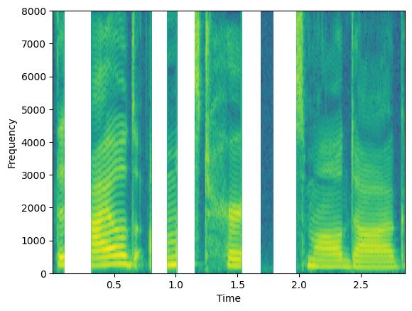
例如，通过设置 parallel_augment=False，选定的增强将按顺序管道应用。相反，如果您选择 parallel_augment=True，每个选定的增强将产生一个不同的增强信号

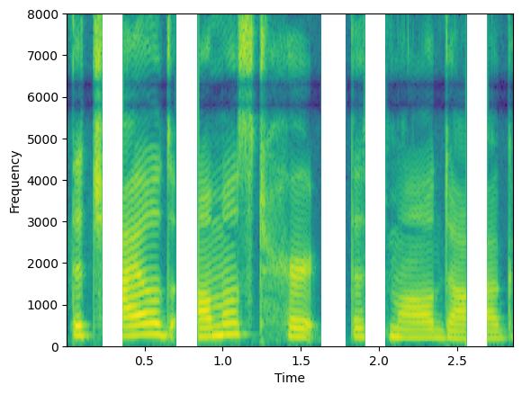
augment = Augmenter(parallel_augment=True, concat_original=False, min_augmentations=2, max_augmentations=2,
                    shuffle_augmentations=False, repeat_augment=1,augmentations=[freq_dropper, chunk_dropper])

augmented_signal, lenghts = augment(clean, lengths=torch.tensor([1.0]))

# We here have two signals, once for each augmentation
print(augmented_signal.shape)

plt.figure(1)
plt.specgram(augmented_signal[0],Fs=16000)
plt.xlabel('Time')
plt.ylabel('Frequency')

plt.figure(2)
plt.specgram(augmented_signal[1],Fs=16000)
plt.xlabel('Time')
plt.ylabel('Frequency')

torch.Size([2, 45920])

/home/sdelang/env/sb312/lib/python3.12/site-packages/matplotlib/axes/_axes.py:8089: RuntimeWarning: divide by zero encountered in log10
  Z = 10. * np.log10(spec)

Text(0, 0.5, 'Frequency')

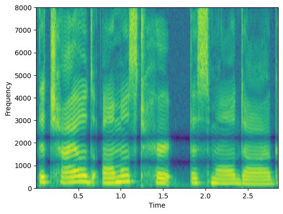
选项 concat_original 参数可用于在输出批量中连接原始信号。

augment = Augmenter(parallel_augment=True, concat_original=True, min_augmentations=2, max_augmentations=2,
                    shuffle_augmentations=False, repeat_augment=1,augmentations=[freq_dropper, chunk_dropper])

augmented_signal, lenghts = augment(clean, lengths=torch.tensor([1.0]))

# We here have three signals: the orignal one + 2 augmentations
print(augmented_signal.shape)

plt.figure(1)
plt.specgram(augmented_signal[0],Fs=16000)
plt.xlabel('Time')
plt.ylabel('Frequency')

plt.figure(2)
plt.specgram(augmented_signal[1],Fs=16000)
plt.xlabel('Time')
plt.ylabel('Frequency')

plt.figure(3)
plt.specgram(augmented_signal[2],Fs=16000)
plt.xlabel('Time')
plt.ylabel('Frequency')

torch.Size([3, 45920])

/home/sdelang/env/sb312/lib/python3.12/site-packages/matplotlib/axes/_axes.py:8089: RuntimeWarning: divide by zero encountered in log10
  Z = 10. * np.log10(spec)

Text(0, 0.5, 'Frequency')

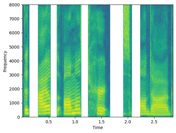
通过操作参数 min_augmentations 和 max_augmentations，我们可以应用可变数量的增强

augment = Augmenter(parallel_augment=False, concat_original=False, min_augmentations=0, max_augmentations=2,
                    shuffle_augmentations=False, repeat_augment=1,augmentations=[freq_dropper, chunk_dropper])

augmented_signal1, lenghts = augment(clean, lengths=torch.tensor([1.0]))
augmented_signal2, lenghts = augment(clean, lengths=torch.tensor([1.0]))
augmented_signal3, lenghts = augment(clean, lengths=torch.tensor([1.0]))

plt.figure(1)
plt.specgram(augmented_signal1.squeeze(),Fs=16000)
plt.xlabel('Time')
plt.ylabel('Frequency')

plt.figure(2)
plt.specgram(augmented_signal2.squeeze(),Fs=16000)
plt.xlabel('Time')
plt.ylabel('Frequency')


plt.figure(3)
plt.specgram(augmented_signal3.squeeze(),Fs=16000)
plt.xlabel('Time')
plt.ylabel('Frequency')

/home/sdelang/env/sb312/lib/python3.12/site-packages/matplotlib/axes/_axes.py:8089: RuntimeWarning: divide by zero encountered in log10
  Z = 10. * np.log10(spec)

Text(0, 0.5, 'Frequency')

在此示例中，我们将 min_augmentations=0 和 max_augmentations=2 与 parallel_augment=False 和 concat_original=False 一起设置。因此，输出可能包含按顺序管道应用的随机数量的增强，范围在 0（无增强）到 2（例如，丢弃频率 + 丢弃分块）之间变化。

通过加入 shuffle=True，可以随机化增强应用的顺序（默认情况下，它遵循增强列表中提供的顺序）。此外，增强管道可以重复多次，生成多个增强信号，这些信号在同一个批量中进行连接。

有关参数的更多详细信息，请参阅 speechbrain.augment 中 Augmenter 类的文档。

参考文献

[1] Daniel S. Park, William Chan, Yu Zhang, Chung-Cheng Chiu, Barret Zoph, Ekin D. Cubuk, Quoc V. Le, SpecAugment: 自动语音识别的简单数据增强方法, Proc. Interspeech 2019, ArXiv

[2] Mirco Ravanelli, Jianyuan Zhong, Santiago Pascual, Pawel Swietojanski, Joao Monteiro, Jan Trmal, Yoshua Bengio: 用于稳健语音识别的多任务自监督学习. Proc. of ICASSP 2020 ArXiv

引用 SpeechBrain

如果您在研究或商业中使用 SpeechBrain，请使用以下 BibTeX 条目引用它

@misc{speechbrainV1,
  title={Open-Source Conversational AI with {SpeechBrain} 1.0},
  author={Mirco Ravanelli and Titouan Parcollet and Adel Moumen and Sylvain de Langen and Cem Subakan and Peter Plantinga and Yingzhi Wang and Pooneh Mousavi and Luca Della Libera and Artem Ploujnikov and Francesco Paissan and Davide Borra and Salah Zaiem and Zeyu Zhao and Shucong Zhang and Georgios Karakasidis and Sung-Lin Yeh and Pierre Champion and Aku Rouhe and Rudolf Braun and Florian Mai and Juan Zuluaga-Gomez and Seyed Mahed Mousavi and Andreas Nautsch and Xuechen Liu and Sangeet Sagar and Jarod Duret and Salima Mdhaffar and Gaelle Laperriere and Mickael Rouvier and Renato De Mori and Yannick Esteve},
  year={2024},
  eprint={2407.00463},
  archivePrefix={arXiv},
  primaryClass={cs.LG},
  url={https://arxiv.org/abs/2407.00463},
}
@misc{speechbrain,
  title={{SpeechBrain}: A General-Purpose Speech Toolkit},
  author={Mirco Ravanelli and Titouan Parcollet and Peter Plantinga and Aku Rouhe and Samuele Cornell and Loren Lugosch and Cem Subakan and Nauman Dawalatabad and Abdelwahab Heba and Jianyuan Zhong and Ju-Chieh Chou and Sung-Lin Yeh and Szu-Wei Fu and Chien-Feng Liao and Elena Rastorgueva and François Grondin and William Aris and Hwidong Na and Yan Gao and Renato De Mori and Yoshua Bengio},
  year={2021},
  eprint={2106.04624},
  archivePrefix={arXiv},
  primaryClass={eess.AS},
  note={arXiv:2106.04624}
}